Lesson#143: How to make a mirror of a table in excel
Hello guys! I am back with a new lesson. Here I will show you to make a formula that can make a mirror of an excel table.
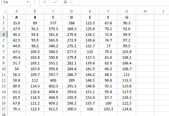
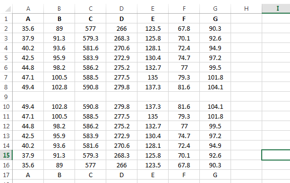
Here I have made a table with some data. I will make a simple formula that will mirror that table horizontally on the left side.
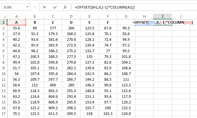
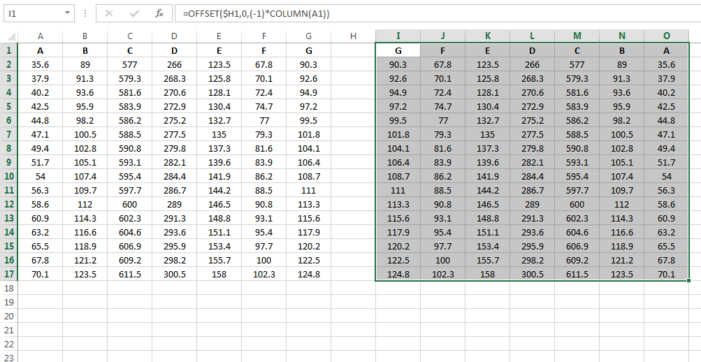
I just put the formula column I =OFFSET($H1,0,(-1)*COLUMN(A1))
What kind of result it is going to return? We will see it in the next picture.
Now how can you make a table mirror vertically?
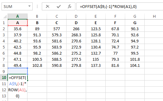
I just put a formula =OFFSET(A$9,(-1)*ROW(A1),0)
If you are having a problem understanding the formula then you must learn these functions.
More examples of Excel function OFFSET
More examples of Excel function ROW
More examples of Excel function COLUMN
Download the example file from the given link below.
See this video to get it clearly.
Hope you liked the tricks to making a mirror of an excel table. These type of tricks are really useful to make your office works more easily. Comment in the comment box below the post to suggest more excel formulas that you need. Visit the YouTube channel Excelabcd to get more useful Excel videos.
Learn excel from here. Get an amazing Excel course from Zero to Intermediate level. Click on the banner below.

Hi! I am Pushpendu. I am the founder and author of Excelabcd. I am little creative person, blogger and Excel-maniac guy. I hope you enjoy my blog.
can u explain how to recreate these formulas as it is not clear? i was able to reform the 2nd one to use it in my sheet but not the first
Download the sheet. I have given link.
This us awsome. Thanks bro