Lesson#116: How to name a range in excel
This post will teach you the basic concept of Name Manager. Here I will show how to name a range in excel.
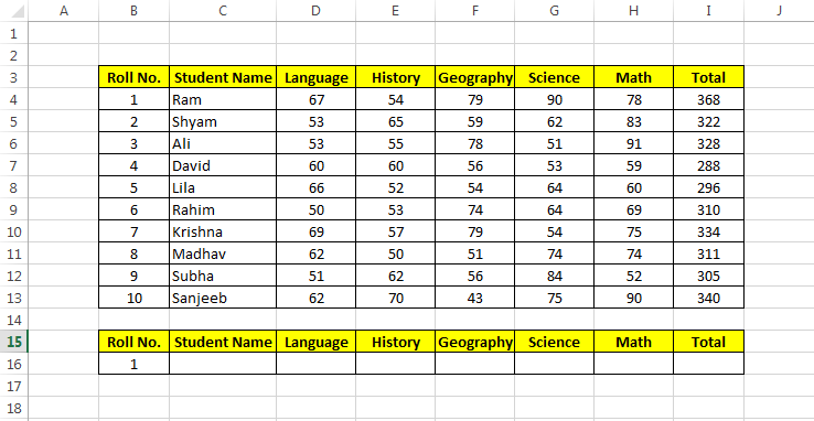
You can also create names for the range, reference, or formula to work in the spreadsheet easily. Above picture shows a simple data table of student marks, and names.
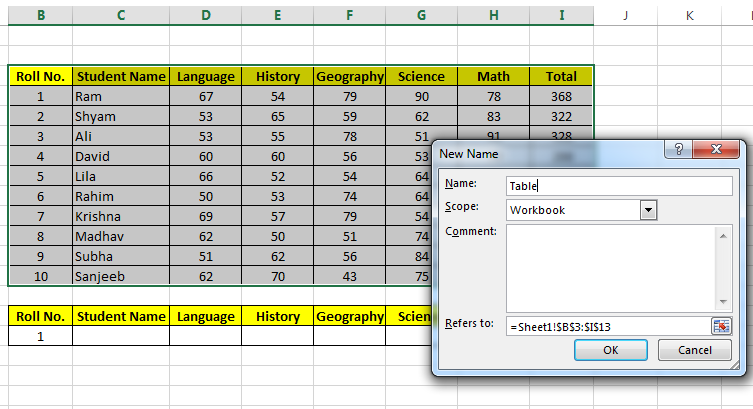
For the easiness of work, we can use names for a range of cells. For that, you have to go to Formulas>Name Manager or simply use the shortcuts Ctrl+F3
Click on the New button then put a desired name for the range and select the range in the Refers to: place.
Like it has shown in the above picture.
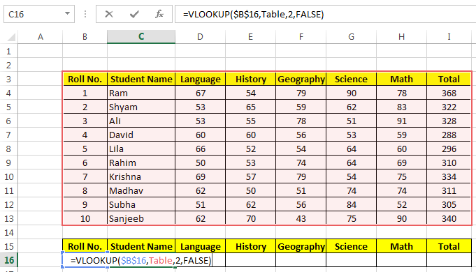
See in the above picture I have used the name ‘Table’ instead of the cell range for the VLOOKUP function. This gives the exact result.
Just like the cell range, we can use names for formulas also.
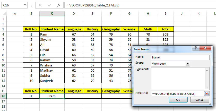
Now I have added another new name where I have put the formula to lookup the student’s name. Please no the point I can use a previously added name in the formula to make a new name.
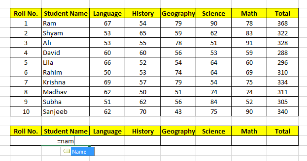
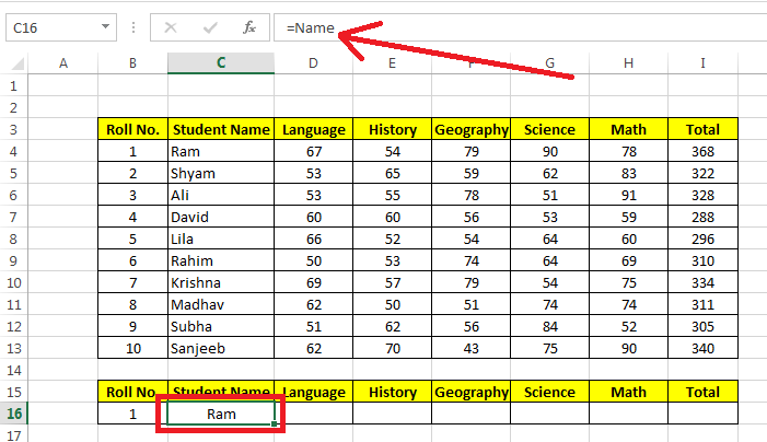
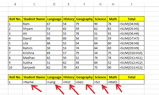
From now every next time I can use only the name after the “=” sign to avoid writing a long formula.
0 Comments on “Lesson#116: How to name a range in excel”