Lesson#115: Information functions with Conditional Formatting

Here I will share general tips about Conditional Formatting and some Information functions. These functions are ISBLANK, ISERR, ISERROR, ISEVEN, ISFORMULA, ISLOGICAL, ISNA, ISNONTEXT, ISNUMBER, ISODD, ISREF, ISTEXT.

You can use these functions to highlight the specified types of values among an array.

ISBLANK function highlights blank cells among an array of values.

ISERR function highlights errors among an array of values.

ISERROR function highlights errors among an array of values.

ISEVEN function highlights even numbers among an array of values.

ISFORMULA function highlights cells if it contains any formula among an array of values.

ISLOGICAL function highlights cells if it contains any logical values among an array of values.

ISNA function highlights cells if it contains any #N/A errors among an array of values.

ISNONTEXT function highlights cells if there are any non-text values among an array of values.

ISNUMBER function highlights cells if there are any number values among an array of values.

ISODD function highlights cells if there is any odd number among an array of values.

ISREF function highlights cells if it contains any reference among an array of values.

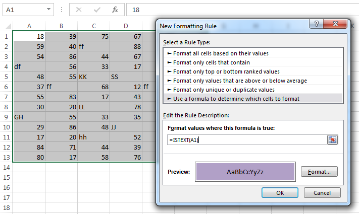
ISTEXT function highlights cells if there are any text values among an array of values.

How to use these functions with Conditional Formatting?

Suppose you are having an array that contains many types of values. Then you have to follow these steps.

1st step: First You have to select the whole array or the area where to highlight and go to Conditional Formatting>New Rule

2nd step: After that select Use a formula to determine which cells to format.

3rd step: Select a format to use by clicking on the Format button.

4th step: Then use the formula in this way. Example: =ISTEXT(A1)=TRUE. Here A1 is the upper left cell or starting cell of the selected area.

Why A1?

You have to put the starting cell in the formula(Most upper left corner). So remember these points whenever you are using the formula in Conditional Formatting.

1. Whenever you are using a formula in Conditional Formatting you have to use the most upper left corner cell reference of the selected array where you apply Conditional Formatting.
2. You never use $ in that cell reference formula.

So If the array starts from cell D10 then the generic formula should use D10.