Lesson#114: How to highlight cells with text or non-text values

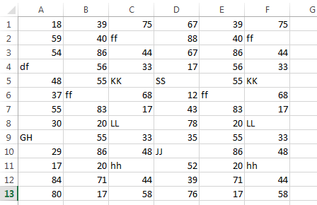
We will discuss how to highlight text values or non-text values among an array. In the above picture, I have shown an example of the array which contains both text and non-text values. What do you have to do when you need to highlight only text values? You have to follow some steps then.

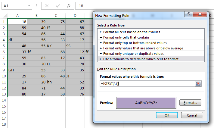
1st step: First You have to select the whole array or the area where to highlight and go to Conditional Formatting>New Rule

2nd step: After that select Use a formula to determine which cells to format.

3rd step: Select a format to use by clicking on the Format button.

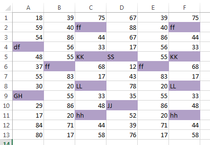
4th step: Then use the formula =ISTEXT(A1)=TRUE. Here A1 is the upper left cell or starting cell of the selected area.

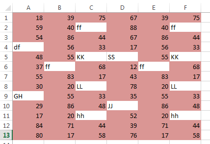
Now I will show you how to highlight non-text values in arrays. You have to follow the same steps as above but there will be a certain change in the formula.

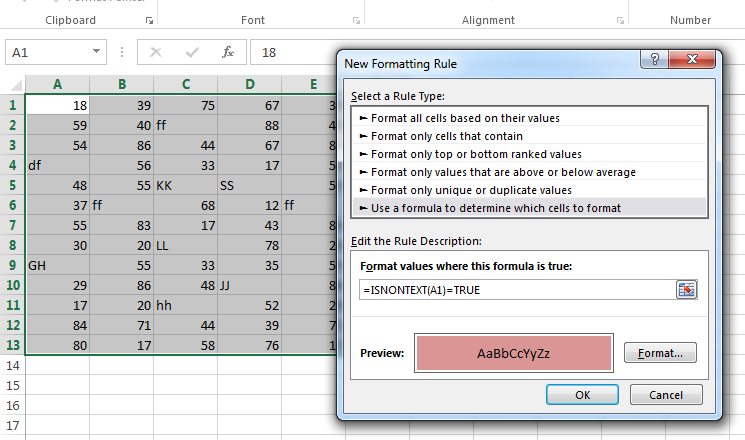
You have to use this formula in Conditional Formatting to highlight non-text values.

=ISNONTEXT(A1)=TRUE.