Lesson#68: COUNTIFS and SUMIFS function in Excel

COUNTIFS is a function to count those cells within a range which meets multiple criteria.Syntax of the function is COUNTIFS(criteria_range1, criteria1, [criteria_range2, criteria2]…)

criteria_range1 – This is the first range to evaluate.
criteria1 – The criteria to be used on criteria_range1.
criteria_range2 – [optional] This is the second range to evaluate.
criteria2 – [optional] The criteria to be used on criteria_range2.

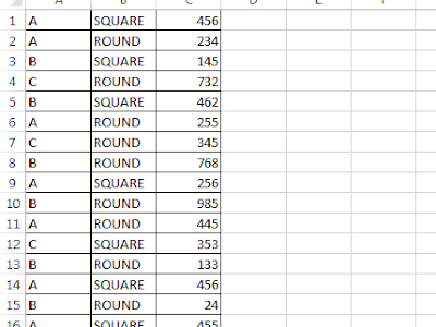
Here I am having a chart like this which I have shown in this picture.

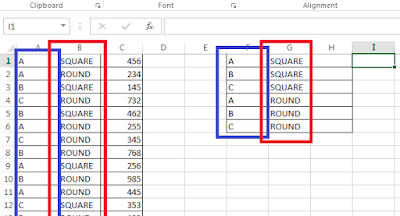
we need to count those items in the A column and B column which meet both of the criteria in the F column and G column.

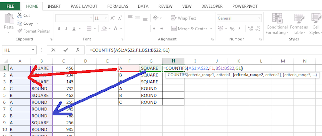
For that, I have used this formula =COUNTIFS(A$1:A$22,F1,B$1:B$22,G1)

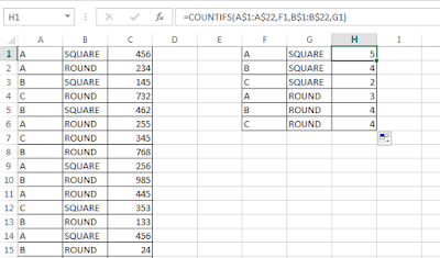
To count cells with multiple criteria we have to use the function COUNTIFS

SUMIFS sums the value of those cells within a range which meets multiple criteria.

Syntax of the function is SUMIFS(sum_range, criteria_range1, criteria1, [criteria_range2, criteria2], …)

sum_range – The range to be summed.
criteria_range1 – This is the first range to evaluate.
criteria1 – The criteria to be used on criteria_range1.
criteria_range2 – [optional] This is the second range to evaluate.
criteria2 – [optional] The criteria to be used on criteria_range2.

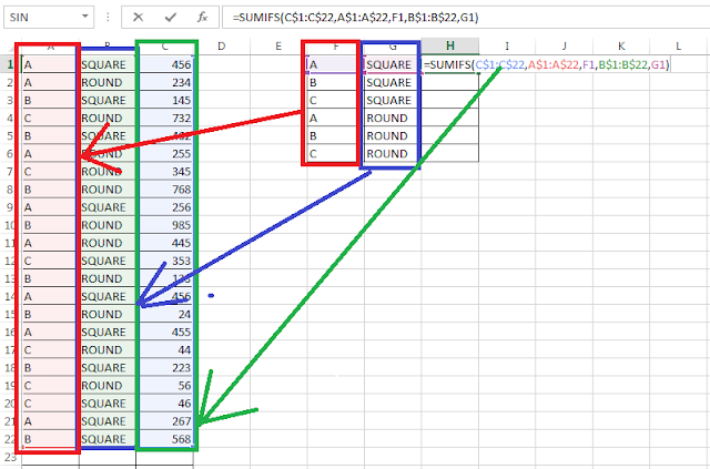
So instead of counting the cells now we need to sum those values in the C column which meets both of the criteria in the A and B columns which are mentioned in the F and G columns.

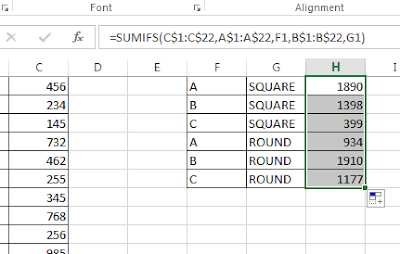
For that I have used this formula =SUMIFS(C$1:C$22,A$1:A$22,F1,B$1:B$22,G1)

To sum cells with multiple criteria, we have to use the function SUMIFS

Related Video Tutorials: