Lesson#49: Make a parent Gantt chart from a data table

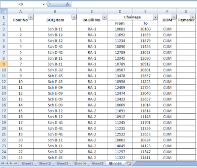
Here I have to make a parent Gantt chart from a data table. It is a Gantt chart summary as per BOQ (Bill of Quantities) Item and RA Bill No. wise. This bar chart will be followed with chainage value on X-axis. This type of Gantt chart becomes very necessary in infrastructure projects like road projects. By this Gantt chart, we are able to know how much length has been billed against the BOQ item, how much length has been duplicated how many times by wrong document entry or manual error.

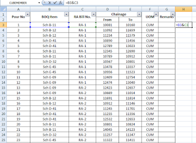
First I have added another column beside the main table and joined the BOQ item and RA Bill No. by using =B3&C3

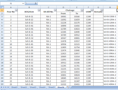
Now I have dragged the formula up to the last entry.

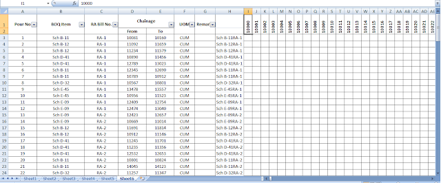
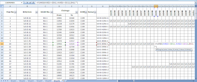
Here I have used this formula =IF(AND(I$1>=$D3, I$1<=$E3),$H3,””). This will reflect data of the H column where chainage value>=From chainage and <=To chainage.

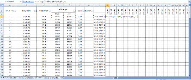
Now I have copied this formula in all cells where I made this dummy Gantt chart.

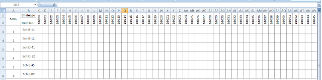
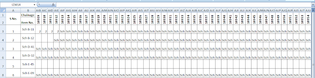
In another sheet (Sheet7), I am making the parent Gantt chart where the data table is to be reflected Item wise and RA Bill No-wise and it has to be presented as a strip chart.

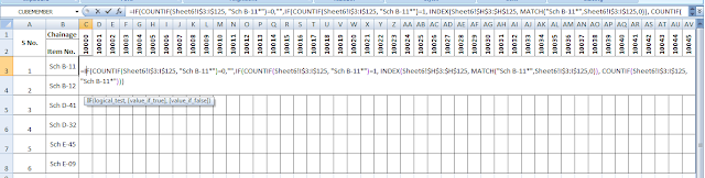
Then I am using this logic for Item no. Sch B-11, this parent Gantt chart will take the data reference from the dummy strip chart. If the count of “Sch B-11*”=0 at Sheet6!I$3:I$125, then it will show “”(blank) or if the count of “Sch B-11*”=1 at Sheet6!I$3:I$125, then it will show the value or text which is in Sheet6 Gantt chart or else the count of “Sch B-11*”>1 at Sheet6!I$3:I$125, it will show the count.
So I have used the formula =IF(COUNTIF(Sheet6!I$3:I$125, “Sch B-11*”)=0,””,IF(COUNTIF(Sheet6!I$3:I$125, “Sch B-11*”)=1, INDEX(Sheet6!$H$3:$H$125, MATCH(“Sch B-11*”,Sheet6!I$3:I$125,0)), COUNTIF(Sheet6!I$3:I$125, “Sch B-11*”))) and copied in the whole row of Sheet7 parent gantt chart.

Using the same logic for Sch B-12, =IF(COUNTIF(Sheet6!I$3:I$125, “Sch B-12*”)=0,””,IF(COUNTIF(Sheet6!I$3:I$125, “Sch B-12*”)=1, INDEX(Sheet6!$H$3:$H$125, MATCH(“Sch B-12*”,Sheet6!I$3:I$125,0)), COUNTIF(Sheet6!I$3:I$125, “Sch B-12*”))) and copied in the whole row of Sheet7 parent gantt chart.

and this way I will put the formula for another item also.  

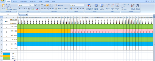
Now the chart looks like the below picture I have shown.

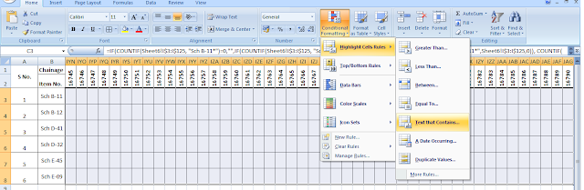
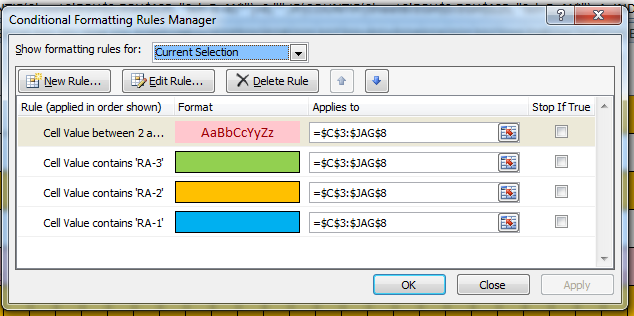
Now I am selecting the Gantt chart area as shown in the picture below and applying conditional formatting Text that Contains and applies different colors for RA-1, RA-2, and RA-3, so it is visible how much length of that item has been claimed in that particular RA Bill.

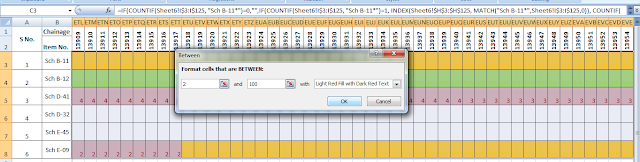
Applying another Conditional Formatting Format cells that are BETWEEN and I have put the values 2 and 100 show it is also visible if the item has been repeated in the same chainage for any data entry error, documentation, or manual error.

My grant chart is working well.

It will make a perfect Gantt chart without any manual coloring error from the data table but it has a disadvantage that the file becomes heavy when it contains more rows on that sheet where the data table is.

It is advisable that in the dummy Gantt chart paste the values of previous entries. In this way, the file will not be heavy.

I have given a download link to the example file which I have shown in this post.

Download