Lesson#48: Graphical 20X20 multiplication table

In this post, I will make a graphical 20X20 multiplication table and show the process of making it.
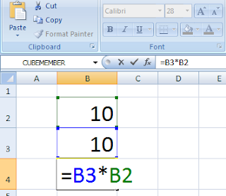
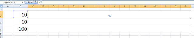
Selected two random numbers between 0 to 20 and multiplied both of them.
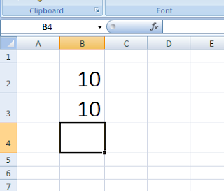
Reflected the cell values in merged cells as I have shown in the picture below.
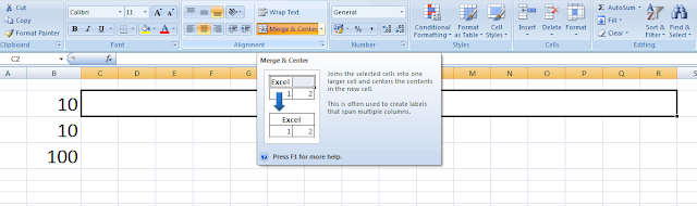
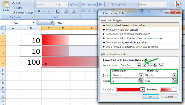
Selected the three merged cells Conditional Formatting>Data Bars>More Rules
Ticked on Show Bar Only checkbox.
Below Shortest Bar and Longest Bar, I have selected the type Number and Shortest Bar value 0,
Longest Bar value is 20X20=400.
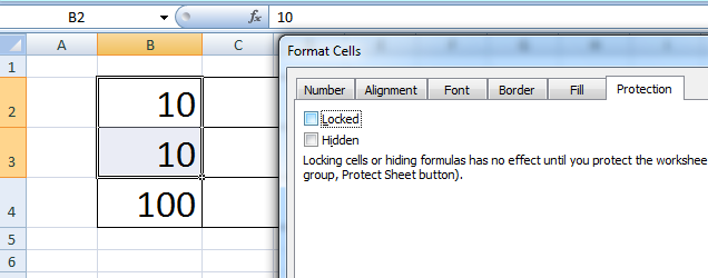
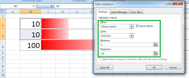
Selected two input cells. Clicked on Data Validation.
Allow>Whole Number.
Minimum: 0
Maximum: 20
Graphical representation of 20×20 multiplication table.
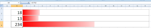
This is a simple example and idea of working with Conditional Formatting. This type of idea can be implemented in your spreadsheet works to make your data presentation more unique.
Hi! I am Pushpendu. I am the founder and author of Excelabcd. I am little creative person, blogger and Excel-maniac guy. I hope you enjoy my blog.