Lesson#29: Explaining CONDITIONAL FORMATTING very simply

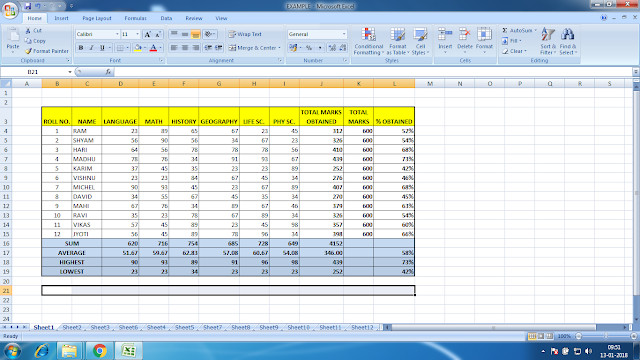
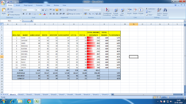
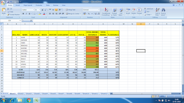
This is an example of a student mark sheet. In this worksheet, I will use the CONDITIONAL FORMATTING option and I will show how it works.

In the CONDITIONAL FORMATTING menu, we get these options

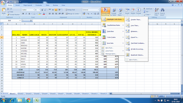
Highlight Cell Rules >
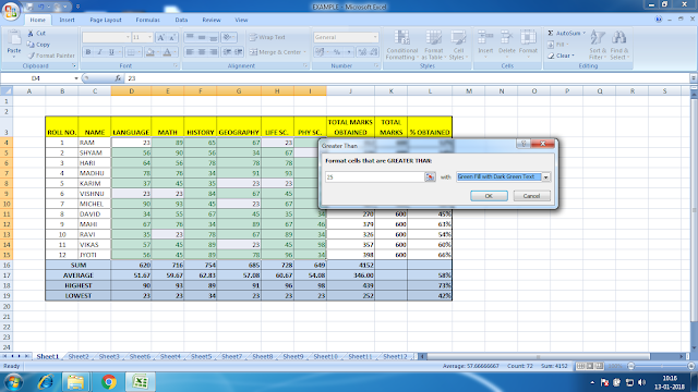
Greater Than… (Highlight those cells having greater than a given value in a given range),
Less Than…(Highlight those cells having lesser than a given value in a given range),
Between…(Highlight those cells having values between two given values in a given range),
Equal to…(Highlight those cells having equal to a given value in a given range),
Text that Contains…(Highlight those cells having any text which is given in a given range),
A Date Occurring…(Highlight those cells having any date occurring which is given in a given range),
Duplicate Values… (Highlight those cells having duplicate or unique values in a given range)

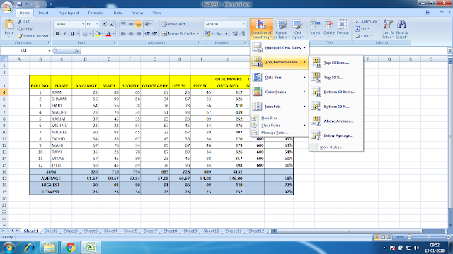
Top/Bottom Rules >
Top 10 Items… (Highlight those cells having top values in a given range),
Top 10%…(Highlight those cells having the top of the given percentage values in a given range),
Bottom 10 Items… (Highlight those cells having bottom values in a given range),
Bottom 10%…(Highlight those cells having the bottom of the given percentage values in a given range),
Above Average… (Highlight those cells having above-average values in a given range),
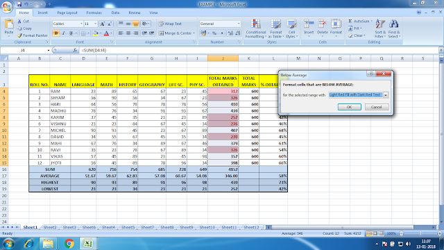
Below Average… …(Highlight those cells having below average values in a given range),

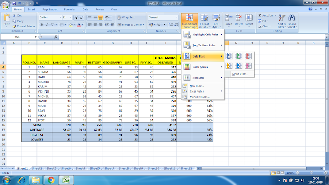
Data Bars>
Creates a data bar within the cell for a graphical representation of the values in a given range.

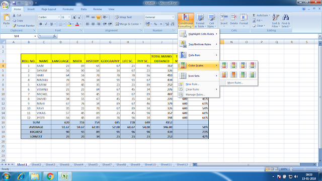
Color Scales>
Creates a color scale within the cell for a graphical representation of the values in a given range.

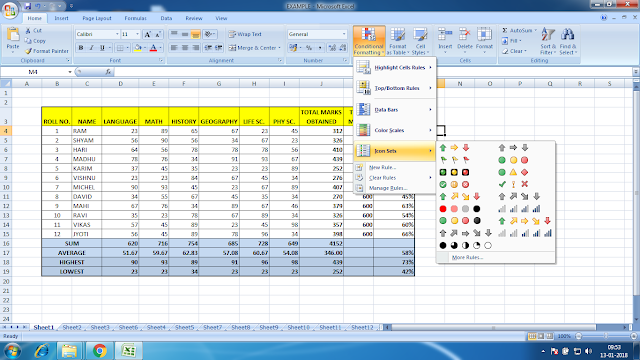
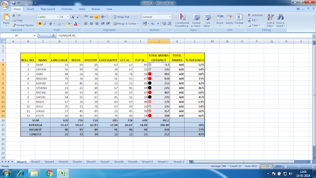
Icon Sets>
Sets icons depending upon the values of the cells in a given range.

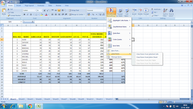
Clear Rules and Manage Rules.

Examples of worksheets using CONDITIONAL FORMATTING.

Highlight Cell Rules >
Greater Than… (Highlight those cells having greater than a given value in a given range),

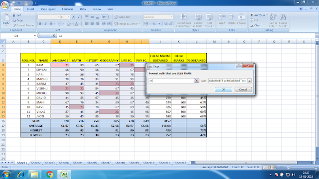
Highlight Cell Rules >
Less Than…(Highlight those cells having lesser than a given value in a given range),

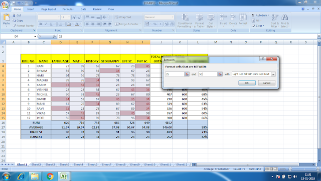
Highlight Cell Rules >
Between…(Highlight those cells having values between two given values in a given range),

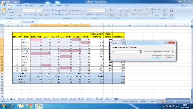
Highlight Cell Rules >
Equal to…(Highlight those cells having equal to a given value in a given range),

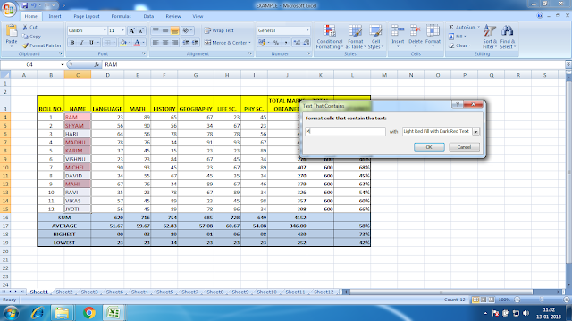
Highlight Cell Rules >
Text that Contains…(Highlight those cells having any text which is given in a given range),

Highlight Cell Rules >
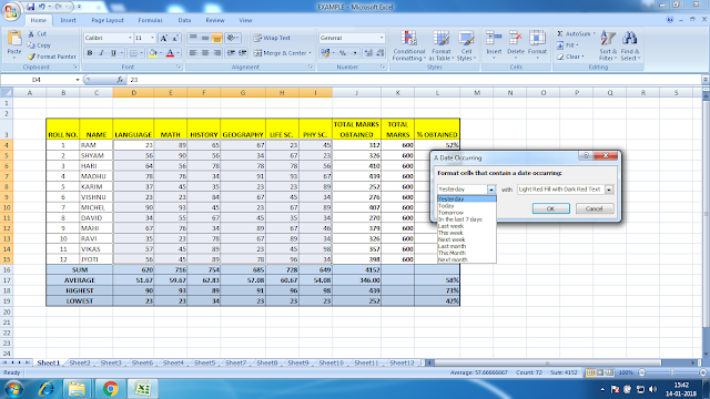
A Date Occurring…(Highlight those cells having any date occurring which is given in a given range),
It will show you a list of highlighting dates that satisfy these criteria, yesterday, today, tomorrow, in the last 7 days, last week, this week, next week, last month, this month, and next month.

Highlight Cell Rules >
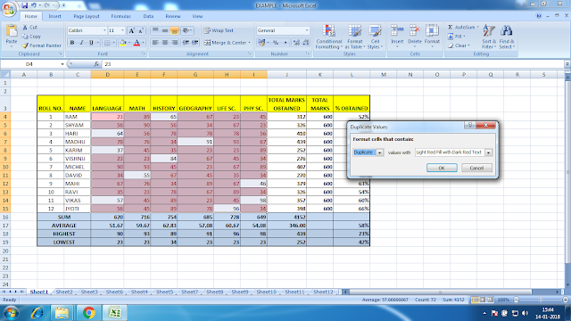
Duplicate Values… (Highlight those cells having duplicate or unique values in a given range)

Top/Bottom Rules >
Top 10 Items… (Highlight those cells having top values in a given range),

Top/Bottom Rules >
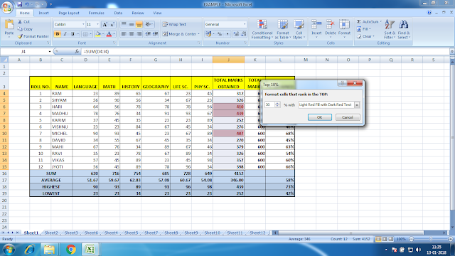
Top 10%…(Highlight those cells having the top of the given percentage values in a given range),

Top/Bottom Rules >
Bottom 10 Items… (Highlight those cells having bottom values in a given range),

Top/Bottom Rules >
Bottom 10%…(Highlight those cells having the bottom of the given percentage values in a given range),

Top/Bottom Rules >
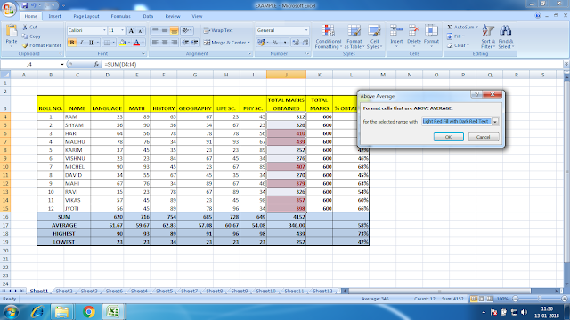
Above Average… (Highlight those cells having above-average values in a given range),

Top/Bottom Rules >
Below Average… …(Highlight those cells having below average values in a given range),

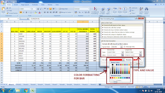
Data Bars>
Creates a data bar within the cell for a graphical representation of the values in a given range.

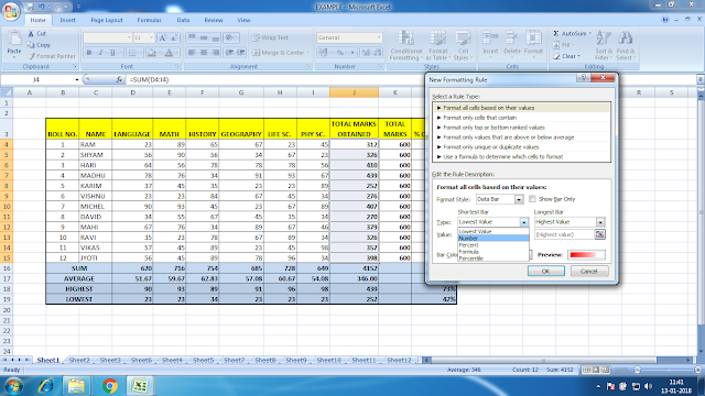
You can select the type of value for making data bars for mentioning the lowest and highest range.

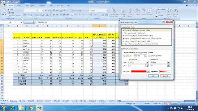
You can select the color of the bar from Bar Color:

This is how it looks when applied. I have selected the range as numbers from 0 to 600. This data bar shows where the values are lying between this range.

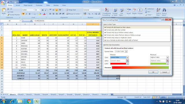
Color Scales>
Creates a color scale within the cell for a graphical representation of the values in a given range.
Like data bar color scale also makes a graphical representation. It changes the color from one another on the basis of the value which lies within a specified range.

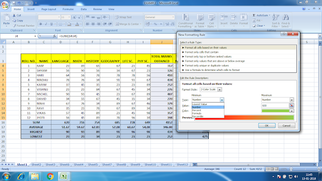
You can select the type of value for making color scales by mentioning the lowest and highest range.

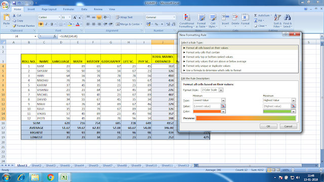
You can select the colors of the lowest and highest values from Color:

This is how it looks when applied. I have selected the range as numbers from 0 to 600. This color scale shows where the values are lying between this range.

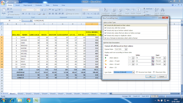
Icon Sets>
Sets icons depending upon the values of the cells in a given range.
3-4 types of icons you can set here depending upon the values.

These are the features of CONDITIONAL FORMATTING in an easy simple way.
There are more options in CONDITIONAL FORMATTING. You can use a formula to format cells in a specified range that meets the formula result.
I will explain it in another post.