Lesson#30: Modify CONDITIONAL FORMATTING by using formula

In my previous post Lesson#29: Explaining CONDITIONAL FORMATTING very simply I explained CONDITIONAL FORMATTING.

In this post, I will show how to modify CONDITIONAL FORMATTING by using a formula.

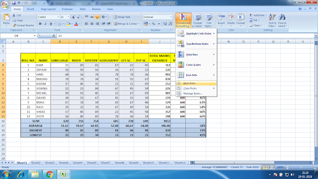
1st you have to select the area where you want to apply CONDITIONAL FORMATTING then click on Conditional Formatting>New Rule

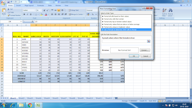
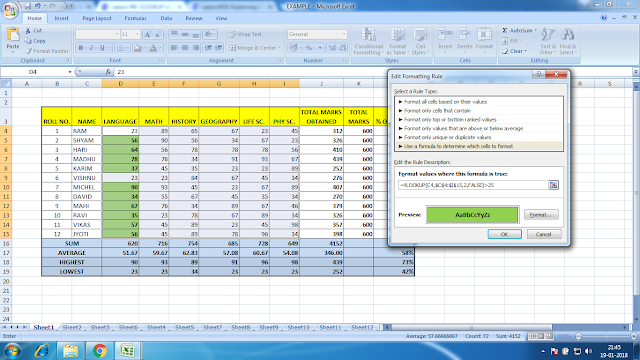
The New Formatting Rule window will open. Here you have to set the format and add a formula below Format values where this formula is truly written.

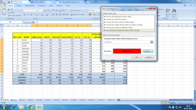
I have entered a formula =D4<8^2. 

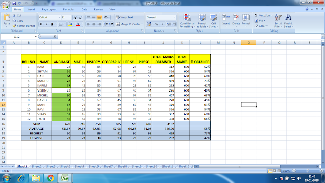
It has formatted those cells where the formula is true.

Here I will show another example where I have put the formula =VLOOKUP(C4,$C$4:$I$15,2,FALSE)>25 

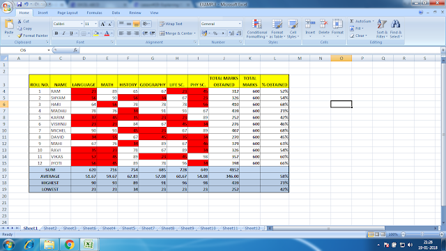
Here is the result.

Note: 1. Formula has to be started with “=”
2. Select the area and go to Conditional Formatting then apply the formula on any one cell (example =D4<8^2. Here D4)