Lesson#2: Making and formatting table, SUM function, and AVERAGE functions

We will learn how to make a table with a simple mark-sheet example and we will learn the Excel SUM and AVERAGE functions.

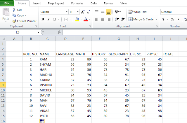
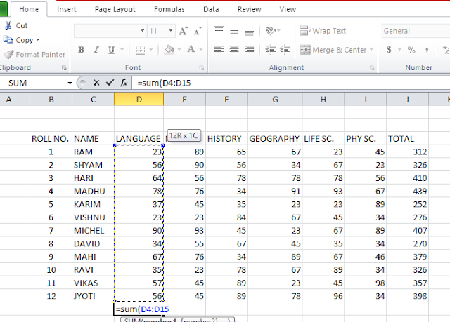
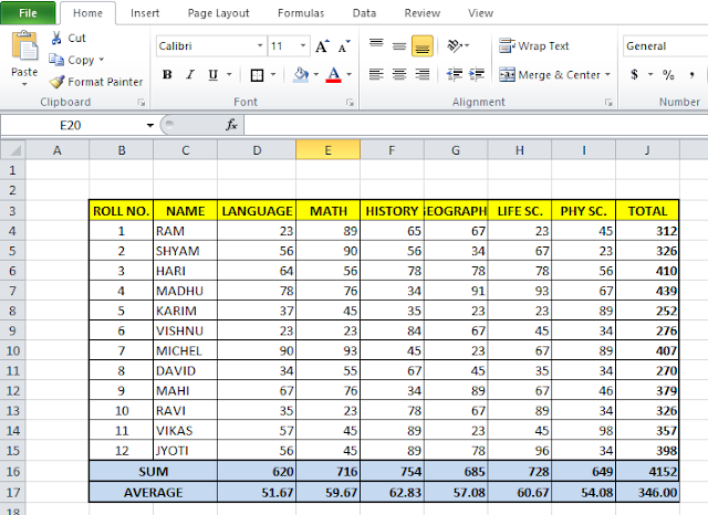
This is a table I have made. On the left side, there are names of students, on top subjects and I have put the marks they have scored against the subject. Now, what do we do? We have to find out the total marks of every student. Should I use the addition method like the previous post? No.

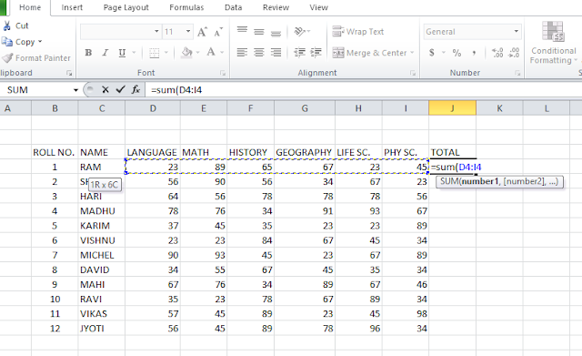
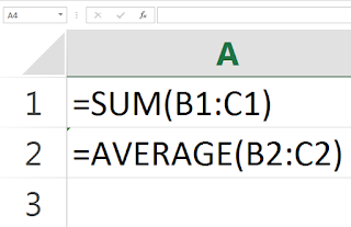
We will use the formula SUM. select the cell type =SUM(select cells). close the bracket. you have to always start with a ‘=’ sign for using a formula.

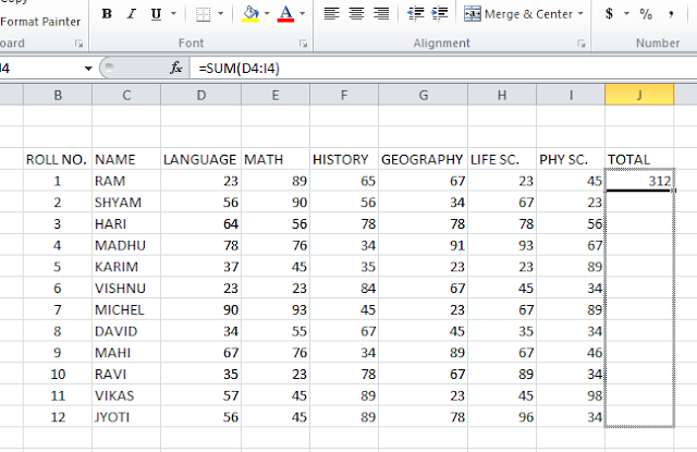
Now we will get the summation of marks. I will click on the corner of the cell and drag it to the bottom row to copy and paste the formula for every student.

Likewise, I will SUM the columns also to check the total score of the class in every subject.

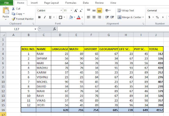
Now I am going to make this table a little presentable. I will format it by selecting all cells and giving borders. I will make the main headers bold and color the bottom and top lines.

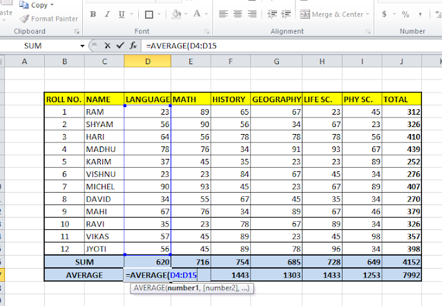
Now I have copied and pasted the bottom row to check the average score in every subject. We have to learn another formula, AVERAGE. now type =AVERAGE(Select the cells) and of course close the bracket.

Now drag in the next cells in the bottom row then we will get average scores in every subject and in total also.

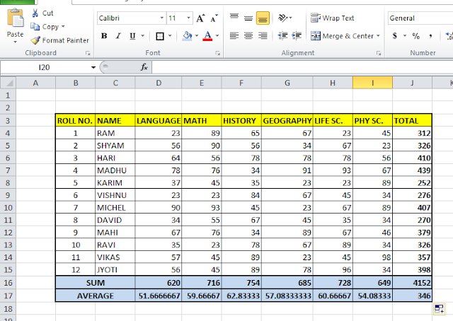
I want to see digits after point only. Then select the cells and click on the button to decrease the decimal. Not good yeah?? This class needs really attention in every subject… Hmm.

Related video tutorials: