Lesson#3: Showing percentage, learning function MAX, function MIN

We made a table of mark sheets in the previous post; now we will learn something new. We will learn to show percentages, the function MAX, and the function MIN

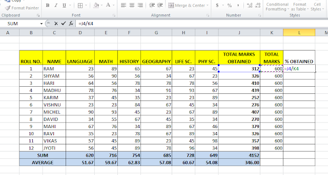
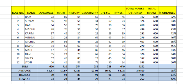
I have added columns on the right-hand side and put total marks there, which is 6*100=600 in every row. Then another column is for showing the percentage of marks scored by each student. Selected the cell and pressed ‘=’, then the total marks obtained cell, then “/” and the total marks cell.

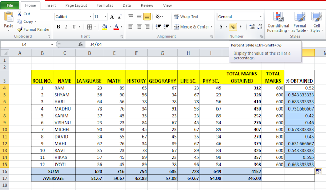
It will show like this in a fraction after a point. I will select all the cells and click on the (%) percent style button and make them bold.

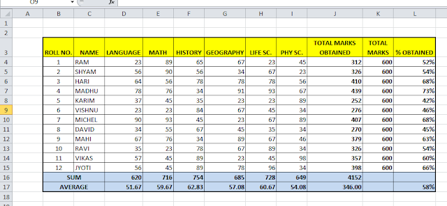
Now, this is what it will look like. Now you can view the percentage of every student and the average percentage scored by the whole class.

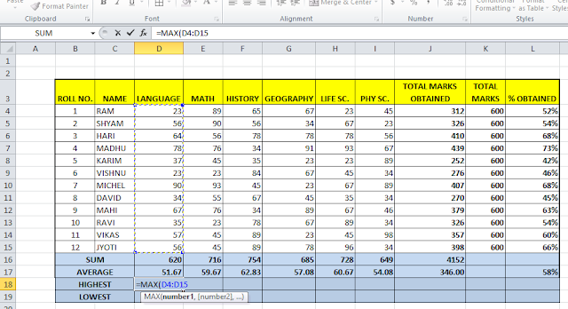
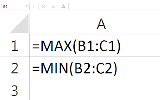
Now we will learn another formula, MAX, to show the highest number. I have added a row at the bottom. Now I want to know what the highest number was in class in every subject. I will type =MAX(select the bottom cell up to the top cell, like the picture) and enter. Then I will drag the formula for every column.

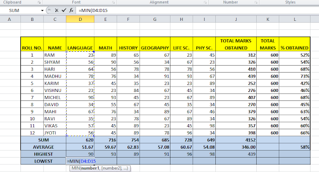
Now another formula, MIN, to show the lowest number. I have added another row at the bottom. Now I want to know what the lowest number was in class in every subject. I will type =MIN(select the bottom cell up to the top cell, like the picture) and enter. Then I will drag the formula for every column.

So we have learned percentage, function MAX, and function MIN successfully. I hope you enjoyed reading my post. Here are some video tutorials for you

Related video tutorials: