Lesson#96: How to HLOOKUP chart from a drop-down menu in Excel

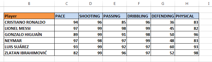
So here is another important lesson for you. How to HLOOKUP chart from a drop-down menu in Excel? Here I am having a table. Table contents skill set data of six players. Here I will show you how to HLOOKUP the chart from there.
First, you have to make a drop-down menu from Data Validation (List).
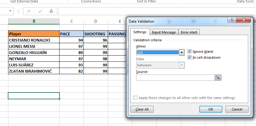
For that, you have to go to Data>Data Validation and then select List below Allow. Clicking on the source button you have to select the skill set name list to insert into the menu.
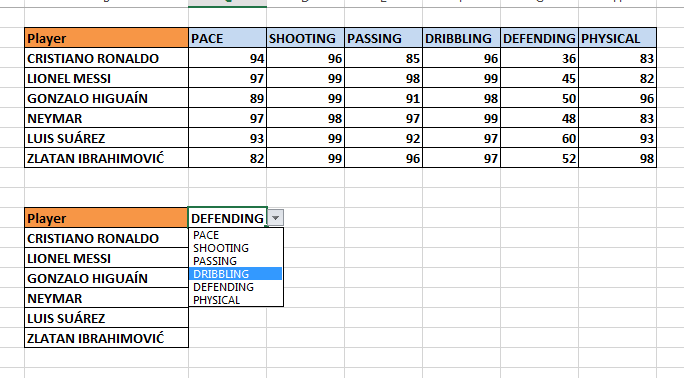
Now your drop-down is ready and I have put the player names in the left column.
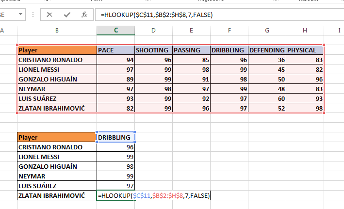
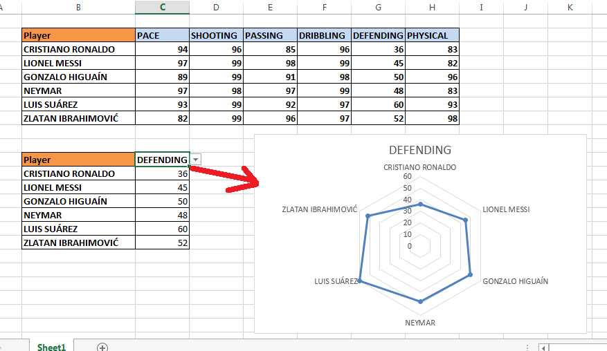
Now you have to HLOOKUP the data from the above table. As I have shown in the above picture.
Now you have to go to Insert>Charts>Insert Stock, Surface, or Radar Chart and then you insert a Radar Chart.
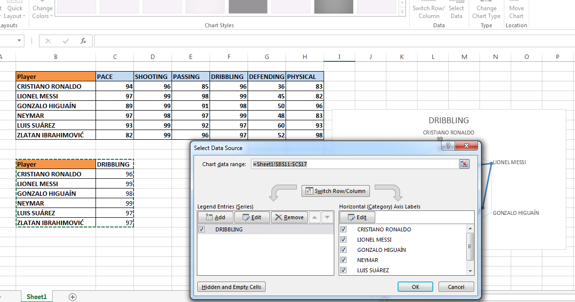
After inserting a blank chart in the worksheet you have to right-click on the chart and click on select data. Click that button beside the Chart data range. Select all the areas where you made HLOOKUP. See the above picture.
Now Enter and click on OK. Now select any skill from the drop-down menu then the chart area will show the chart for the selected skill only and for all players. So that is how to HLOOKUP chart from a drop-down menu in Excel.
If you like this post then please share it on social media and don’t hesitate to subscribe to the blog by email.
Hi! I am Pushpendu. I am the founder and author of Excelabcd. I am little creative person, blogger and Excel-maniac guy. I hope you enjoy my blog.