Lesson#95: How to VLOOKUP chart from a drop-down menu in Excel

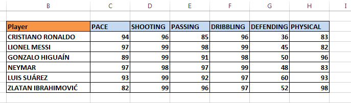
So that’s an important lesson for you my dear. How to VLOOKUP chart from a drop-down menu in Excel? Here I am having a table. Table contents skill set data of six players. Here I will show you how to VLOOKUP the chart from there.

First, you have to make a drop-down menu from Data Validation (List).

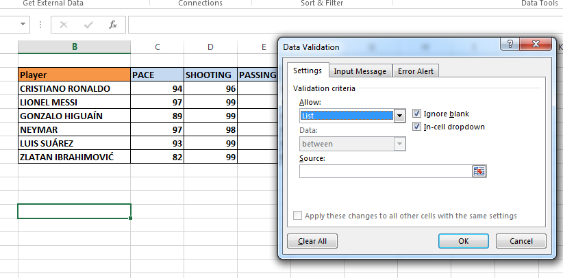
For that, you have to go to Data>Data Validation and then select List below Allow. Clicking on the source button you have to select the player’s name to insert into the menu.

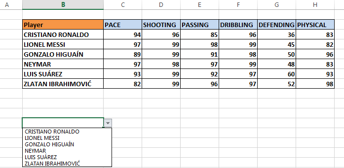
See, now the drop-down menu list is ready.

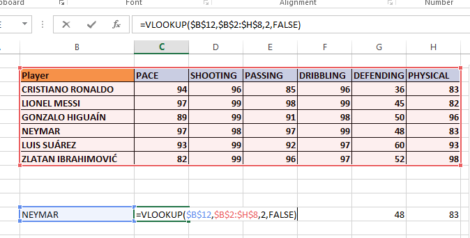
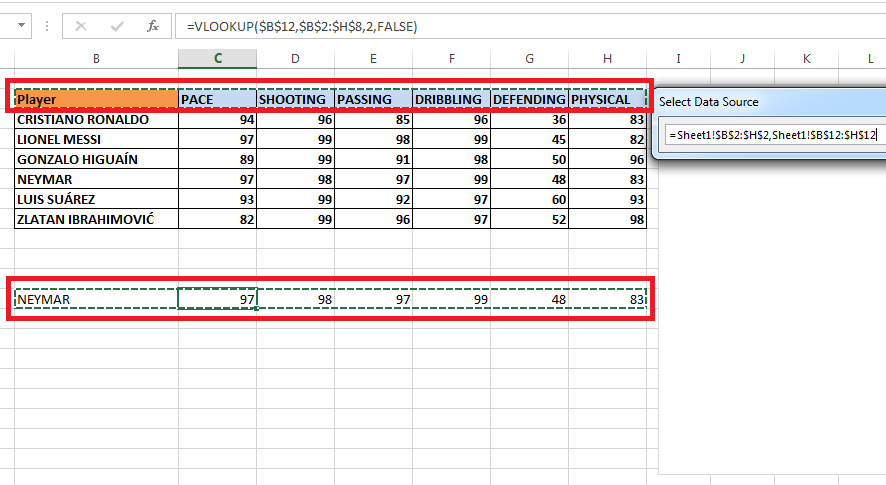
Now you have to VLOOKUP the data from the above table. As I have shown in the above picture.

Now you have to go to Insert>Charts>Insert Stock, Surface, or Radar Chart and then you insert a Radar Chart.

After inserting a blank chart in the worksheet you have to right-click on the chart and click on select data. Click that button beside the Chart data range. By pressing Ctrl 1st select the Label area then select the Value area where you made VLOOKUP. See the above picture.

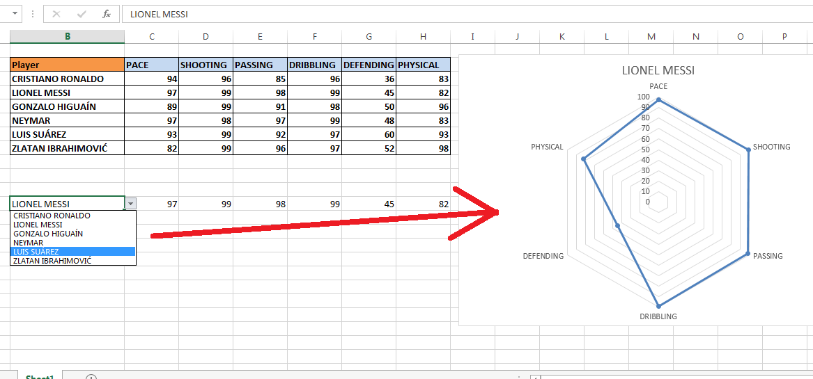
Now Enter and click on OK. Now select any name from the drop-down menu then the chart area will show the skill chart for the selected player only. So that is how to VLOOKUP chart from a drop-down menu in Excel.

If you like this post then please share it on social media and don’t hesitate to subscribe to the blog by email.