Lesson#113: How to highlight cells with errors in it

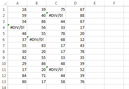
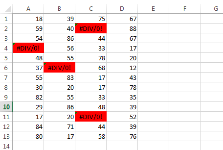
I will show you how to highlight cells with errors among an array of values. Here I am having an array of values and among them, I have some cells which contain errors. If you need to highlight those cells only which are having errors in it then follow these steps.

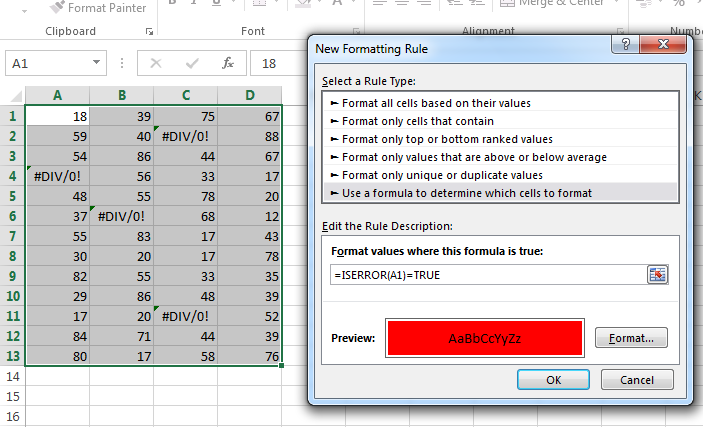
1st step: First You have to select the whole array or the area where to highlight and go to Conditional Formatting>New Rule

2nd step: After that select Use a formula to determine which cells to format.

3rd step: Select a format to use by clicking on the Format button.

4th step: Then use the formula =ISERROR(A1)=TRUE. Here A1 is the upper left cell or starting cell of the selected area.