Lesson#19: How to convert digit into word in excel

In this lesson, we will learn a method to convert digits into words. I will use functions like CONCATENATE, VLOOKUP, SUM, IF, and MOD, which were discussed in my previous posts.

1st Step

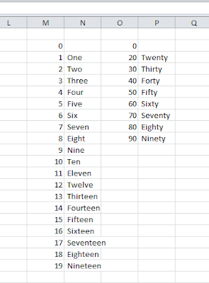
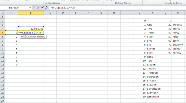
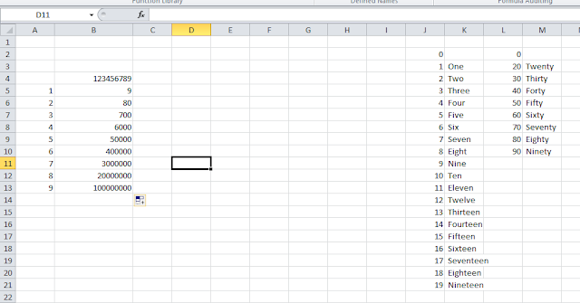
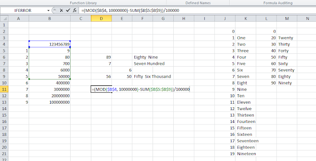
For example, I have taken the number 123456789 and I am making a chart. In the first column, I have put 1 to 9. In the second column, I have added the formula at cell B5 =MOD($B$4, 10^A5) beside 1 which will show the remainder after diving the number by 10^1.

3rd Step

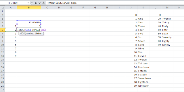
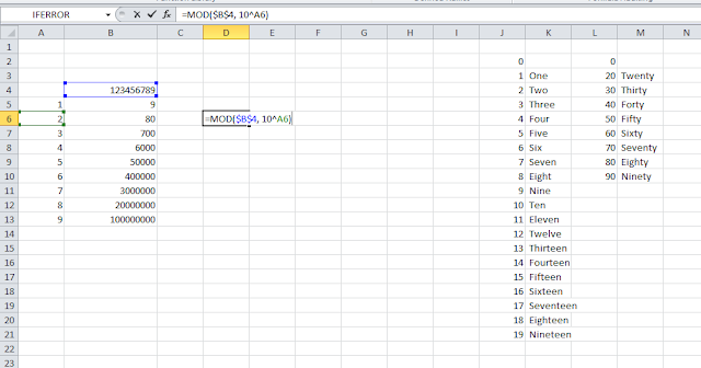
At the next cell B6 =MOD($B$4, 10^A6)-$B$5 beside 2 which will show the result of subtraction between the remainder after diving the number by 10^2 and B5.


4th Step

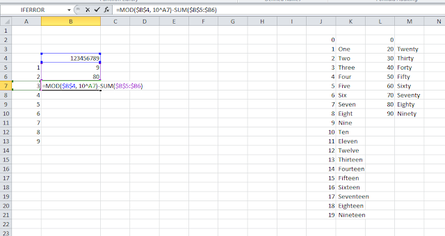
At the next cell B7 =MOD($B$4, 10^A7)-SUM($B$5:$B6) beside 3 which will show the result of subtraction between the remainder after diving the number by 10^3 and the sum of the previous cell to B5.

5th Step

I have dragged the formula up to the 9th cell.

6th Step

At cell D6 I am putting the formula =MOD($B$4, 10^A6) or =MOD($B$4, 100)which will show the remainder after dividing the number by 10^2 or 100.

7th Step

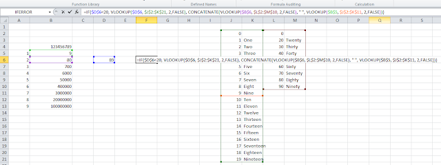
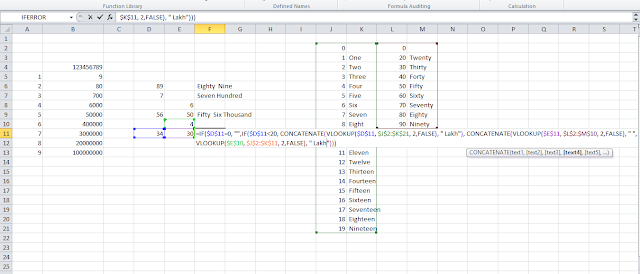
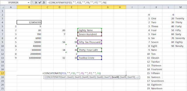
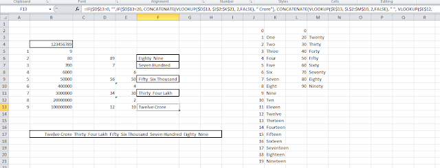
Now I will input the logic when the D6 is less than 20 it will look up the phrase for 0 to 19 and when it will be equal to 20 or larger then it will combine the lookup value for B6 and B5. This is the formula =IF($D$6<20, VLOOKUP($D$6, $J$2:$K$21, 2,FALSE), CONCATENATE(VLOOKUP($B$6, $L$2:$M$10, 2,FALSE), ” “, VLOOKUP($B$5, $J$2:$K$11, 2,FALSE)))

8th Step

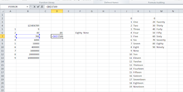
The next step will be for Hundred. At D7 I will put the value of =$B$7/100. 

9th Step

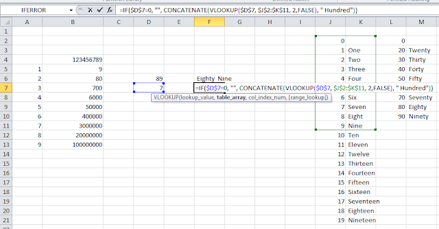
For spelling it I will put the formula =IF($D$7=0, “”, CONCATENATE(VLOOKUP($D$7, $J$2:$K$11, 2,FALSE), ” Hundred”)) 

10th Step

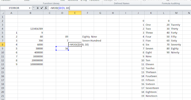
For spelling the Thousand portion I have to extract the two-digit number by using =(MOD($B$4, 100000)-SUM($B$5:$B$7))/1000. At E8  I have put the formula =MOD($D$9, 10)
11th Step

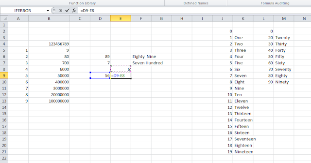
At E9 I have put the formula =D9-E8.
12th Step

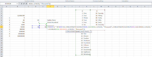
Now the logic is if the value of D9 is less than 20 then it will lookup the phrase for 0 to 19 chart and add “Thousand” as a suffix, else it will concatenate the phrase for E9 and E8 then will add “Thousand” as a suffix. The formula is =IF($D$9=0, “”,IF($D$9<20, CONCATENATE(VLOOKUP($D$9, $J$2:$K$21, 2,FALSE), ” Thousand”), CONCATENATE(VLOOKUP($E$9, $L$2:$M$10, 2,FALSE), ” “, VLOOKUP($E$8, $J$2:$K$11, 2,FALSE), ” Thousand”))). When D9 will be zero then it will be silent.


13th Step

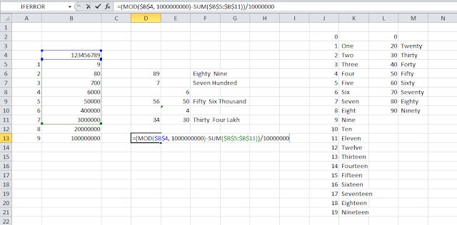
Like the previous steps for spelling Thousand, I will put a formula for Lakhs. For spelling the Lakh portion I have to extract the two-digit number by using =(MOD($B$4, 10000000)-SUM($B$5:$B$9))/100000. 


14th Step

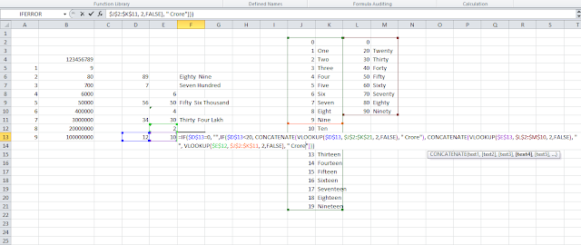
Now the logic is if the value of D11 is less than 20 then it will lookup the phrase for 0 to 19 chart and add “Lakh” as a suffix, else it will concatenate the phrase for E11 and E10 then will add “Lakh” as a suffix. The formula is =IF($D$11=0, “”,IF($D$11<20, CONCATENATE(VLOOKUP($D$11, $J$2:$K$21, 2,FALSE), ” Lakh”), CONCATENATE(VLOOKUP($E$11, $L$2:$M$10, 2,FALSE), ” “, VLOOKUP($E$10, $J$2:$K$11, 2,FALSE), ” Lakh”))). When D11 will be zero then it will be silent.
15th Step

Download this sheet.