Lesson#109: Tricks to make a dancing chart in excel

Here I will show you a funny trick to make a dancing chart in excel.

For that, you have to follow some steps.

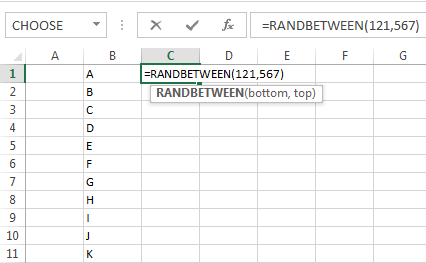
1. Make a range of data names like A, B, C, and D…..

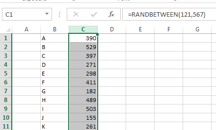
2. Then put values against these names with the RANDBETWEEN formula by putting any arbitrary lower and upper values.

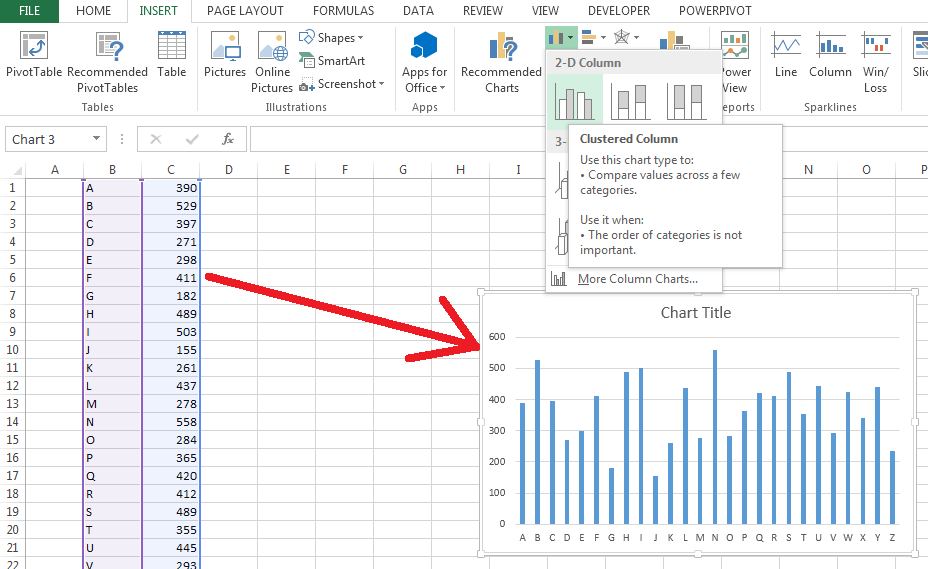
3. Then select the whole data and insert a chart.

Now I will add some simple VBA to make the clock auto refreshed every second. So I have taken these simple steps.

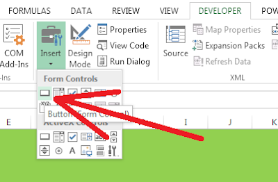
4. From the Developer Tab I have inserted a Button (Form Control) and clicked on New in the Assign Macro window

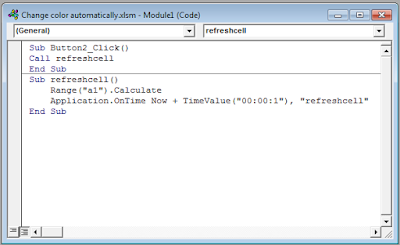
5. Opening the VBA editor I added this code

Sub Button2_Click()
Call refreshcell
End Sub
Sub refreshcell()
Range(“a1”).Calculate
Application.OnTime Now + TimeValue(“00:00:1”), “refreshcell”
End Sub

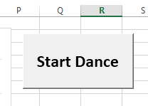
6. Edited the button text and the size just looks good.

7. Save this sheet as a macro-enabled workbook in .xlsm format.

Now see every second this sheet is auto-refreshing the clock. I put that button to call the function refreshcell()
if the sheet doesn’t start to refresh itself automatically after opening it.