Lesson#92: How to highlight a column value depending upon the other column values

Hello Friend! I am back again with my other post. This post is about Conditional Formatting. Here I will show how to highlight a column value depending on the column values next to it.

In the above picture, I am giving you a column with date values and beside this column, you will have another column with number values. You need to highlight the dates if the numerical values besides the dates are between 40 and 45.

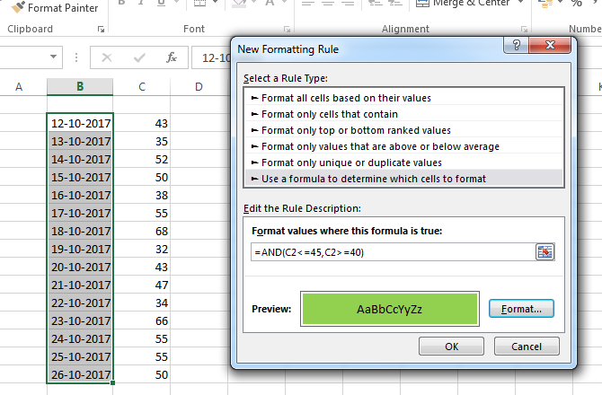
So for that you have to go to Conditional Formatting>New Rule>Use a formula to determine which cells to format

Here you select a format just like the above picture and type this formula =AND(C2<=45,C2>=40)

Here C2 is the first cell in the column upon which we apply the formula.

1. Whenever you are using a formula in Conditional Formatting you have to use the most upper left corner cell reference of the selected array where you apply Conditional Formatting.
2. You never use $ in that cell reference formula.

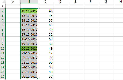
So here is your problem solved. You have successfully highlighted those cells beside which the number value is between 40 and 45.