Lesson#90: How to highlight a particular number in an array automatically

So here I will show you a simple but very useful trick with Conditional Formatting. This is about how to highlight a particular number in an array automatically.

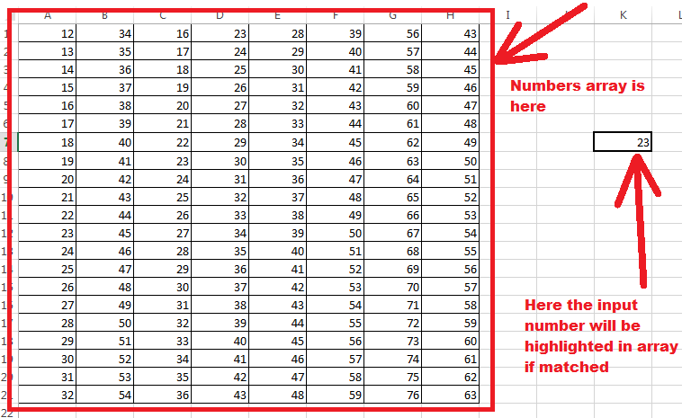
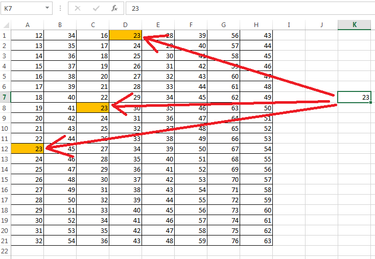
So in the above picture, I have a number array where I will highlight the numbers which will match the number shown in the cell outside of the array. For that, you have to use a simple and very easy method in Conditional Formatting.

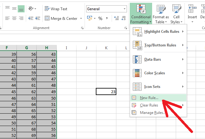
Selecting all the cells in the array you have to go to Conditional Formatting>New Rule as it has shown in the above picture.

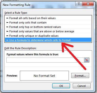
There you have to select the option Use a formula to determine which cells to format.

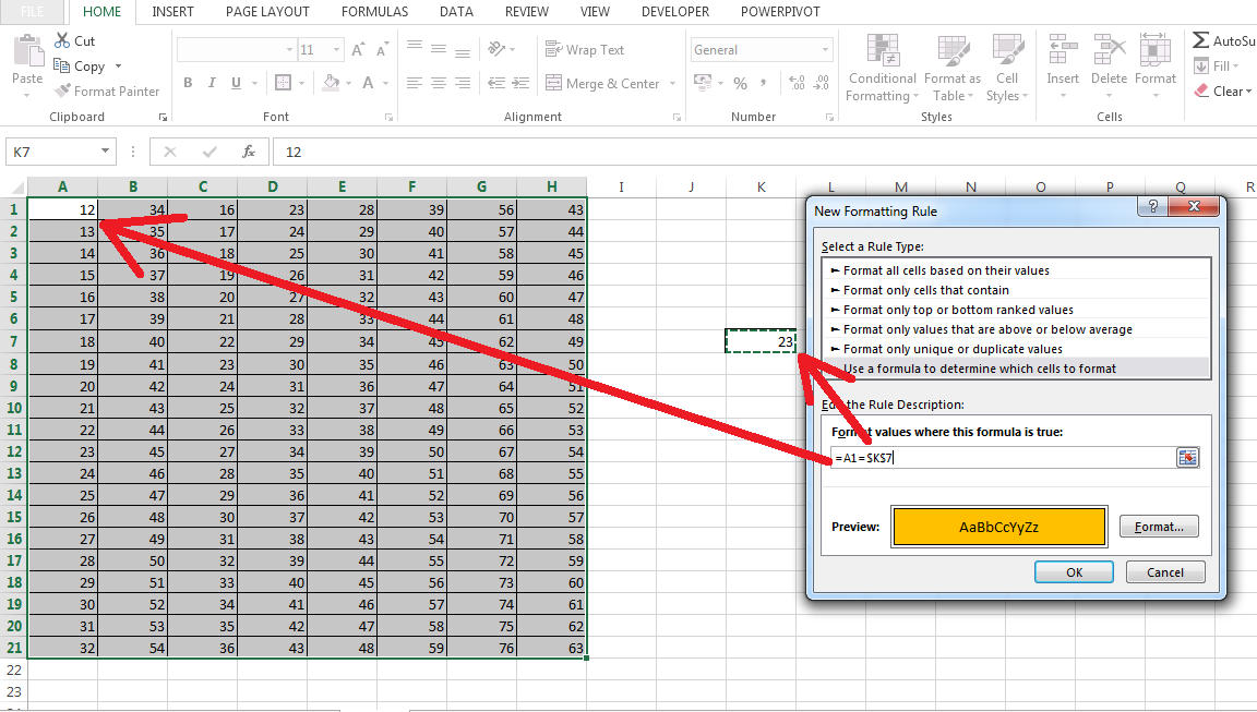
So here the cell where you will input a value to match in the array is K7. Then you have to put this formula in the bar (Format values where this formula is true:) =A1=$K$7

Why A1?

You have to put the starting cell in the formula(Most upper left corner). So remember these points whenever you are using the formula in Conditional Formatting.

1. Whenever you are using a formula in Conditional Formatting you have to use the most upper left corner cell reference of the selected array where you apply Conditional Formatting.
2. You never use $ in that cell reference formula.

So friend next time I will be back with more interesting lessons in Excel. Don’t forget to subscribe to my blog and leave a comment if you like my post.

Related Video Tutorials: