Lesson#64: Freeze panes must be kept in mind

Freeze Panes is a very important feature that is required in spreadsheets. It’s better to keep it always in mind. It allows you to freeze rows or columns or both when you are scrolling down or scrolling right throughout the spreadsheet.

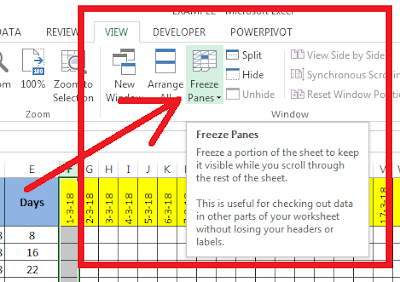
Go to the VIEW tab of the ribbon and here you will find  Freeze Panes. 

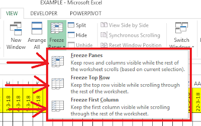
Clicking on the item shows you three options, Freeze Panes, Freeze Top Row, and Freeze First Column.

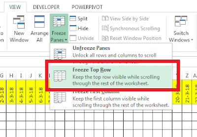
When you need to freeze the top row only you can select Freeze Top Row.

This option freezes the top row even if you scroll down to the bottom of the spreadsheet.

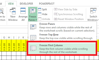
When you need to freeze the first column only you can select Freeze First Column.

This option freezes the first column when you scroll right through the spreadsheet.

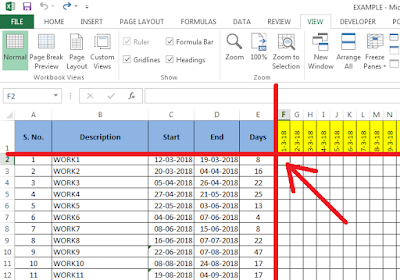
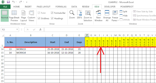
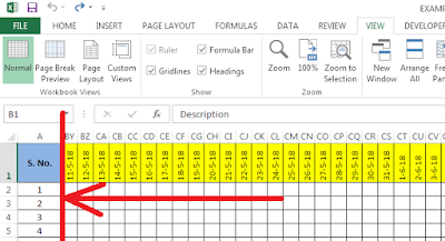
Choose the option Freeze Panes when you want the viewer to be frozen from any column or row or both. (Example:- If you want the viewer to be frozen from column E then select column F click on Freeze Panes, If you want the viewer to be frozen from row 5 then select row 6 and click on Freeze Panes.)


When you want both columns and rows to be frozen click on the intersecting cell which is just at bottom of the rows to freeze and just at the right of the columns to freeze like it as shown in the picture left.

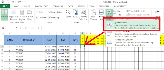
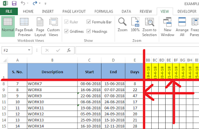
Then click on the Freeze Panes and columns and rows both will freeze when you scroll down or scroll right.