Lesson#53: Simple trick to color all the Sundays in the list of dates at once

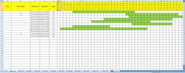
Select all the dates then go to Conditional Formatting>New Rule>Use a formula to determine which cells to format
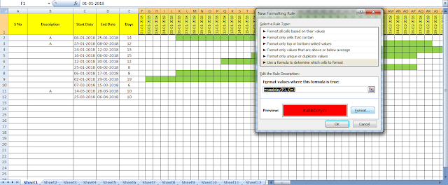
Now I used the formula =WEEKDAY(F1,1)=1 It will color only those dates which are Sundays.
This thing you have to remember when applying formulas in conditional formatting.
You have put the starting cell in the formula, among the selected cells upon which you are applying conditional formatting. So remember these points whenever you are using the formula in Conditional Formatting.
- Whenever you are using a formula in Conditional Formatting you have to use the most upper left corner cell reference of the selected array where you apply Conditional Formatting.
- You never use $ in that cell reference formula.
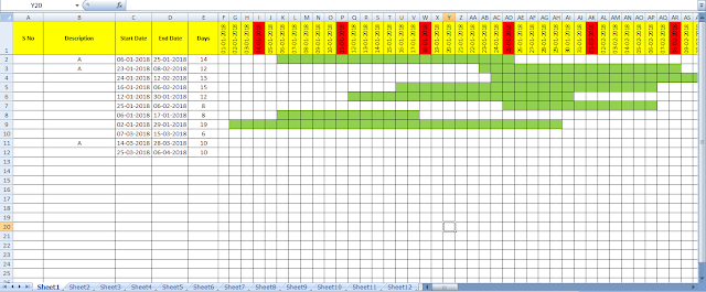
See it’s done here. This is how to color all the Sundays in the list of dates at once with conditional formatting.
Related Video Tutorials:
Hi! I am Pushpendu. I am the founder and author of Excelabcd. I am little creative person, blogger and Excel-maniac guy. I hope you enjoy my blog.