In this post, we will learn to make a calendar which will take input of month from 1 (JAN) to 12 (DEC) and year in numeric format and show the whole month calendar.
1st Step:
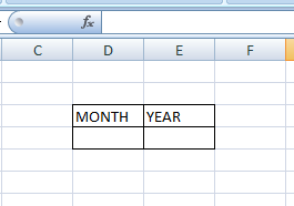
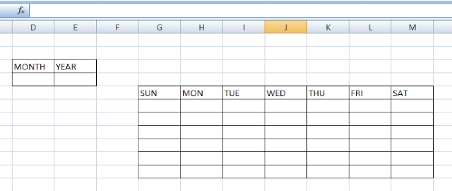
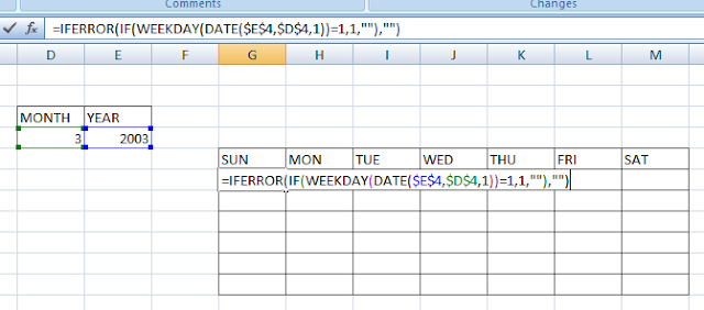
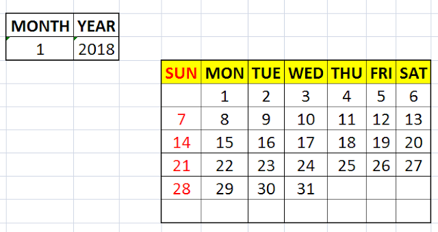
Make a 2×2 table like shown in the picture for entering the value of month and year.
2nd Step:
Now make a 7×7 table for showing the calendar like shown in the picture.
Now the purpose is to show the 1st date of the month below that day of the week on which it actually comes in the calendar.
3rd Step:
In the first row, first column I have put this formula =IFERROR(IF(WEEKDAY(DATE($E$4,$D$4,1))=1,1,””),””).
Logic is to take out the WEEKDAY of DATE(“Year given by user”, “Month given by user”, 1). If this value is 1 then it will show below SUN or it will just show “” (blank).
4th Step:
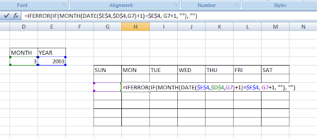
Now the purpose is to (+)1 the next cell of which the day “1” starts.
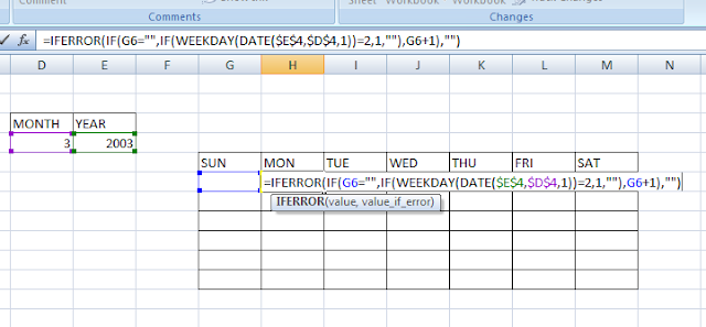
In the next cell we will change the formula a little
=IFERROR(IF(H5=””,IF(WEEKDAY(DATE($F$3,$E$3,1))=2,1,””),H5+1),””). If the previous cell is left “” (blank) then it will take out the WEEKDAY of DATE(“Year given by user”, “Month given by user”, 1). If this value is 2 then it will show below
MON or it will just show “” (blank). In any other case,
IFERROR will be triggered to show “” (blank).Likewise below the
TUE formula is
=IFERROR(IF(H5=””,IF(WEEKDAY(DATE($F$3,$E$3,1))=3,1,””),H5+1),””).
below the
WED formula is
=IFERROR(IF(H5=””,IF(WEEKDAY(DATE($F$3,$E$3,1))=4,1,””),H5+1),””).
below the THU formula is =IFERROR(IF(H5=””,IF(WEEKDAY(DATE($F$3,$E$3,1))=5,1,””),H5+1),””).
below the FRI formula is =IFERROR(IF(H5=””,IF(WEEKDAY(DATE($F$3,$E$3,1))=6,1,””),H5+1),””).
below the
SAT formula is
=IFERROR(IF(H5=””,IF(WEEKDAY(DATE($F$3,$E$3,1))=7,1,””),H5+1),””).
5th Step:
Now the purpose is to show the dates from the 2nd row of the calendar.
SUN will (+)1 SAT date and before showing either the month (+)1 date is equal to the month provided by the user or it left “” (blank). This function will make the calendar show up to the last date of the month whatever is entered by the user. I have used the formula =IFERROR(IF(MONTH(DATE($E$4,$D$4,M6)+1)=$E$4, M6+1, “”), “”)
Similarly in the same row it will (+)1 the previous date using this formula =IFERROR(IF(MONTH(DATE($E$4,$D$4,G7)+1)=$E$4, G7+1, “”), “”).
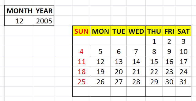
Now I will make the calendar formatted a little to look better.
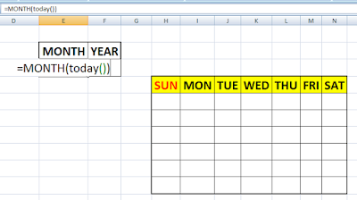
I will make it a little change to show a dynamic calendar which will show only the present month of today’s date.
In the month cell, I will add the formula =MONTH(TODAY()) which will always show the month of TODAY()
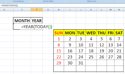
In the year cell, I will add the formula =YEAR(TODAY()) which will always show the year of TODAY()
Now it is a dynamic calendar for the current month.
Download the excel file from the link given below.


I’d have to verify with you here. Which isn’t something I normally do! I enjoy reading a put up that may make people think. Also, thanks for permitting me to remark!
Thanks. Keep following my blog
I’ve read a few good stuff here. Certainly worth bookmarking for revisiting. I surprise how much effort you put to make such a excellent informative website.
Thank you for your comments. Though this website is new but I am trying my best to make it very useful for my all readers. Your nice comments are prize for my work. Always keep revisiting to this site. Thank you.