Lesson#11: How to use the HLOOKUP function in Excel?

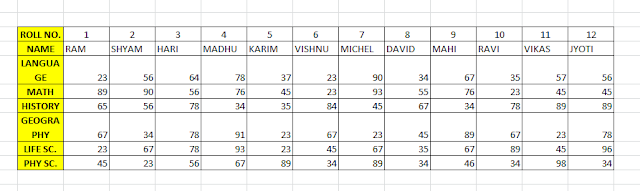
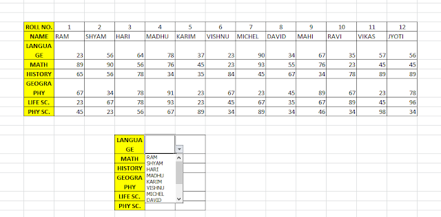
Below the main table, I made a small table to look up the value or marks against the subject name for any student. For time-saving I have made drop-down menu of student names by using data validation.

Structure of HLOOPKUP is HLOOKUP(lookup_value,table_array,row_index_num,range_lookup)

• lookup_value: value to look for — can be a value or a cell reference.
• table_array: lookup table — range reference or a range name, with 2 or more columns.
• row_index_num: row in the lookup table, with value to be returned
• [range_lookup]: for an exact match, use FALSE or 0; for the approximate match, use TRUE or 1, with lookup value row sorted in ascending order

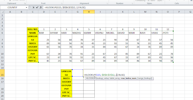
Now I will put this formula =HLOOKUP(G15, $D$6:$O$12, 2, FALSE), where G15 cell is the name of the student, $D$6:$O$12 is the first row from where it will match the student name and 2 is the row number of the selected array for Language subject.

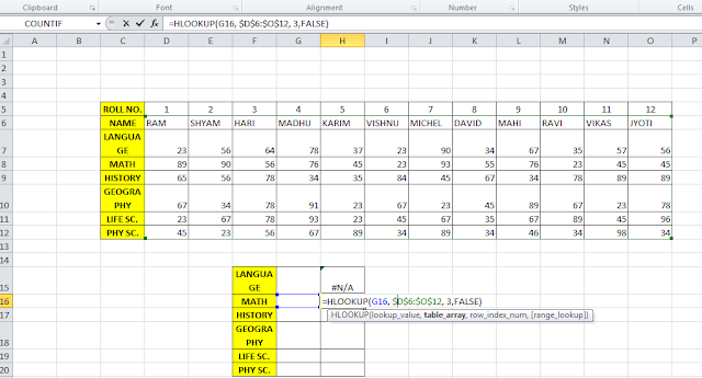
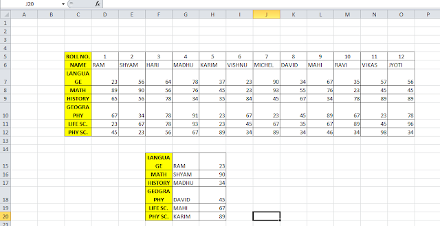
Now you can see the result. You are now able to check marks for any subject of any individual student by using the HLOOKUP function.

Related video tutorials: