Lesson#161: How to remove duplicates in Excel? | 5 ways to delete duplicates in Excel

Maximum Microsoft Excel users frequently ask this question about Excel. One of the most asked questions about Excel is, “How to remove duplicates in Excel?” or “How to delete duplicates in Excel?” or “How do I delete duplicates in Excel but keep one?”. Today I shall answer these questions and I shall show you 5 ways to delete duplicates in Excel in this post.

Method#1: Remove duplicate numeric values with Function MODE and MODE.MULT

What is the Excel MODE function?

The Excel MODE function returns the most frequently occurring value of a number set. It helps you to find a duplicate value in an array.

Syntax of this function is MODE(number1, [number2], …)

where number1 is a number or cell reference that refers to numeric values and

number2  [optional] is A number or cell reference that refers to numeric values.

Example:

=MODE(23,21,21,56,78,99)=21

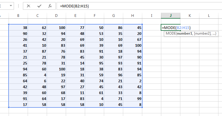
In this above example MODE returned the most frequently occurring value 45. The limitation is it only returns a single value.

What is the Excel MODE.MULT function?

Excel MODE.MULT function returns the most frequently occurring numbers in a numeric data set with a vertical array.

The syntax of this function is MODE.MULT(number1, [number2], …)

where number1 is a number or cell reference that refers to numeric values and

number2  [optional] is a number or cell reference that refers to numeric values.

Example:

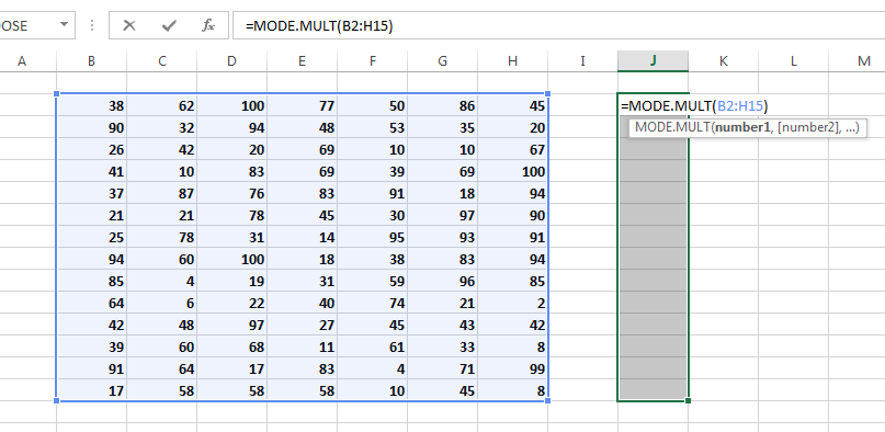
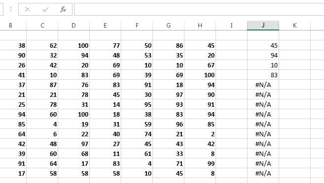
Selected a vertical space in the worksheet then I entered the formula by pressing Ctrl Shift Enter

The limitation of these functions is they return the most occurring values.

What about the duplicate values which occur lesser times?

Method#2: Remove duplicate values in Excel with Conditional Formatting.

Conditional Formatting allows you to find out the duplicate or unique values in a worksheet with a very easy method.

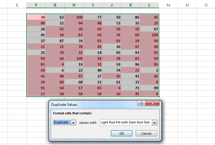
You have to first select the array or the area of the worksheet then go to Conditional Formatting>Highlight cells rules>Duplicate values

There you can select both duplicate and unique values to highlight.

Method#3: Delete duplicate values in Excel with PivotTable.

Here I am showing you an example of how to find duplicates by PivotTable.

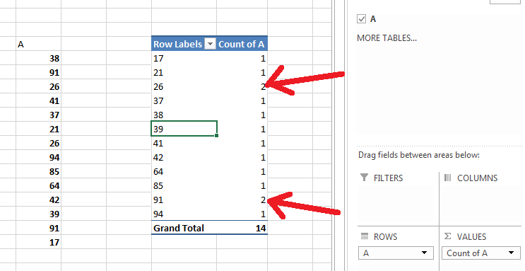
Select the data array and insert a PivotTable. Put the value field in Rows and again put the same field in Values and change the field settings to Count. See there is a nice way to find out.

Method#4: Remove duplicate values in Excel with the COUNTIF function.

You can use COUNTIF and put it in a column beside the array to show how many times it occurs in the complete array.

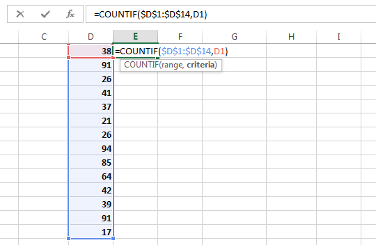
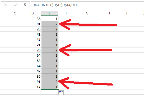
See the above example I have put the COUNTIF function to count the number of times it occurring in an array.

Method#5: Delete duplicates with ‘Remove Duplicates’

There is another good and easy feature of Excel, Remove Duplicates.

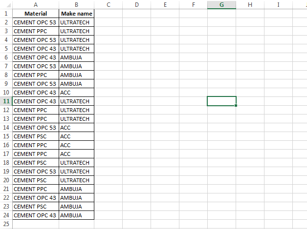
See the above picture I made a list of names of cement and making companies for example. These names are used repeatedly in these two columns. Suppose we need to remove all the duplicate values from one column then we can select the column and just click on Data>Remove Duplicates

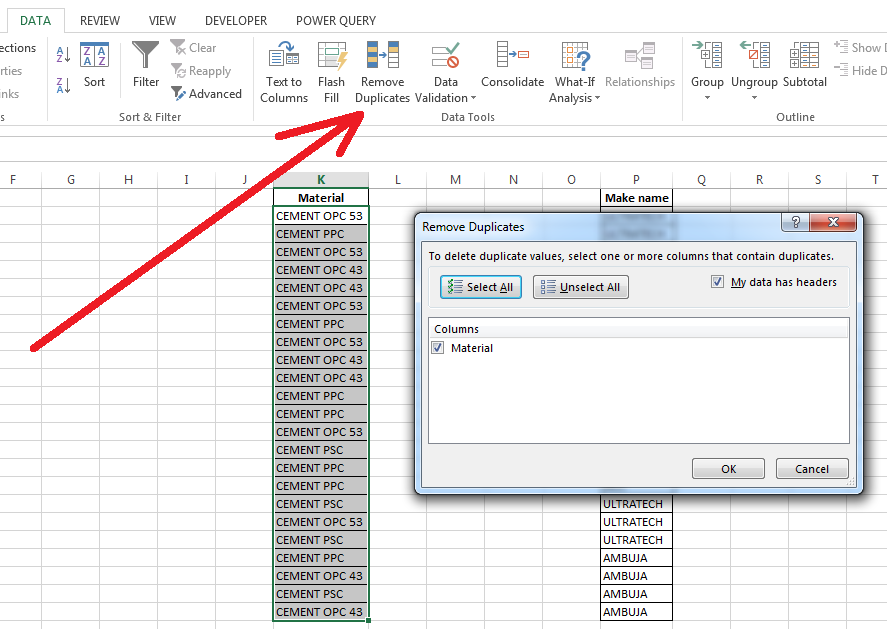
See in the above picture I have selected the option My data has headers so the column is named Material. Now just click on the OK button.

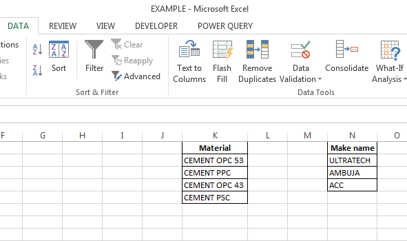
Now if we need to remove the duplicate values by keeping the data combination of multiple columns (For Example CEMENT OPC 53 in column A and ULTRATECH in column B together is a unique value). Then select both columns and then go to Data> Remove Duplicates.

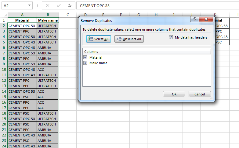
Now just click the OK button.

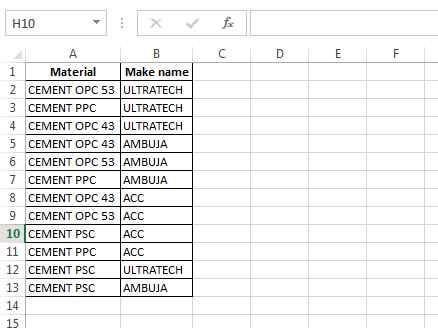
So these are the 5 ways to remove duplicates in Excel.

Join our Telegram channel https://t.me/excelabcd

Here you shall be regularly updated with Excel tips and tricks.