Lesson#132: How to make the function SUMPRODUCTIF

In this post, I will show you the trick to make the function SUMPRODUCTIF. We have the SUMPRODUCT function in excel. But how to make a SUMPRODUCT function that follows criteria like SUMIF?

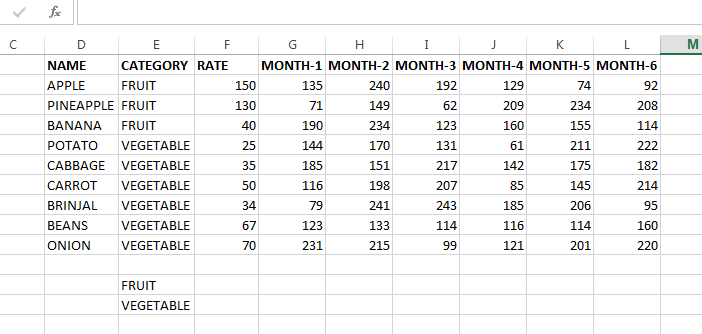
Here I have made an example.

Here’s how to make the function SUMPRODUCTIF.

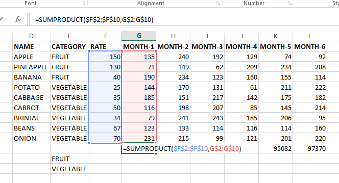
Here’s the total value of all items that can be found by SUMPRODUCT. But if I want to find the total value category wise then I need to modify the formula.

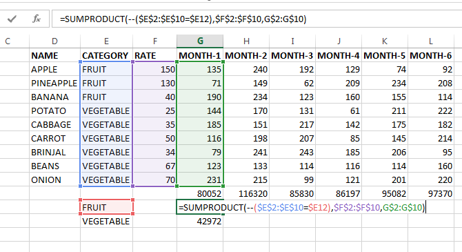
Here it is making SUMPRODUCT for the FRUIT category only.

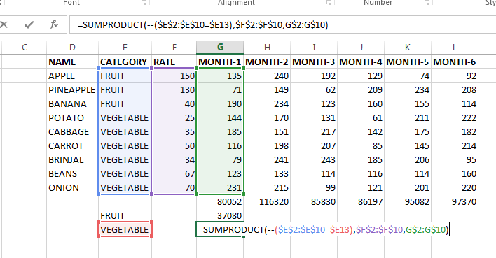
And here it is making SUMPRODUCT for the VEGETABLE category only.

Instead of using this formula =SUMPRODUCT($F$2:$F$10,G$2:G$10) I have used formula =SUMPRODUCT(–($E$2:$E$10=$E12),$F$2:$F$10,G$2:G$10)

What is the Double negative (“–“) do?

Double unary converts the conditions in text value to act like a numeric one and forces the rest of the function to work properly considering the conditions.

This is how to make function SUMPRODUCTIF.

We will discuss more double unary in the next posts.

Download the file from here.