Lesson#43: Make an ON/OFF switch for Conditional Formatting in your excel sheet

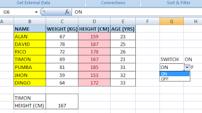
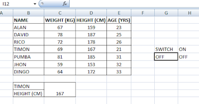
Showing a random example worksheet where I have used conditional formatting and color formatting. Now I will make a switch that will trigger the Conditional Formatting ON or OFF. Besides the table, I have made a drop-down list of ON/OFF with Data Validation.
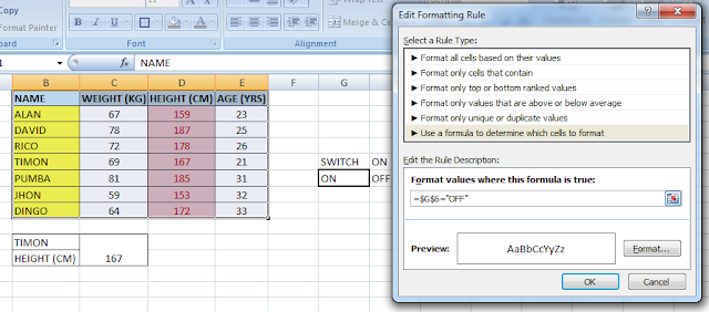
Now I selected the area and clicked on Conditional Formatting>New Rule>Use a formula to determine which cell to format
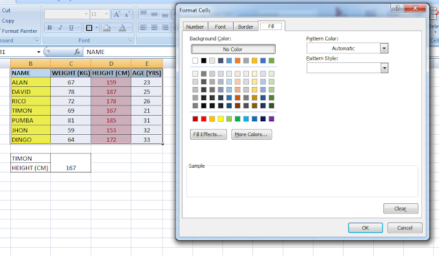
Clicking on Format… I selected No Color on the Fill tab.
Then I put the formula =$G$6=”OFF” to apply this formatting whenever the value of cell G6 is “OFF”.Then I clicked OK.
Now select the area I clicked on Conditional Formatting>New Rule>Manage Rule Select the =$G$6=”OFF” rule and move it to the top. And tick on the Stop If True checkbox.
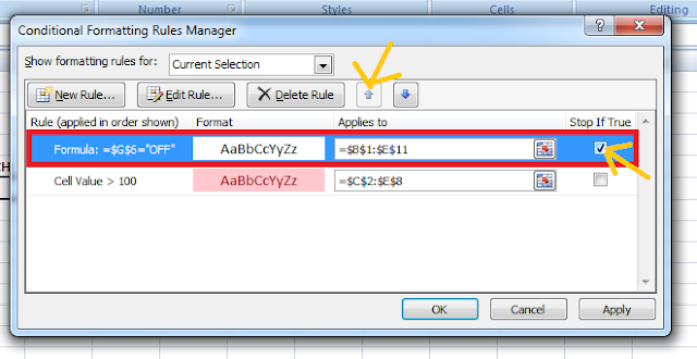
Your Conditional Formatting switch is ready to work.
Video Tutorials:
Hi! I am Pushpendu. I am the founder and author of Excelabcd. I am little creative person, blogger and Excel-maniac guy. I hope you enjoy my blog.