Lesson #9: VLOOKUP explained

In this post function, VLOOKUP is explained here once more with a very simple example.
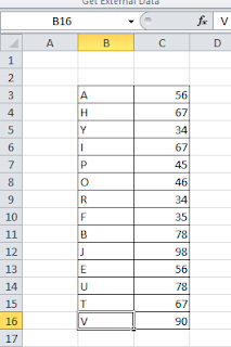
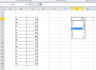
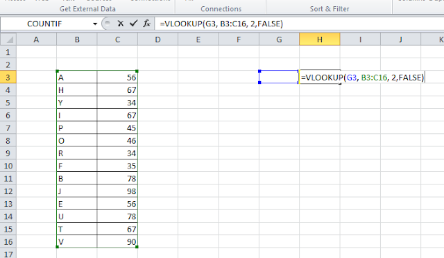
Now, In the above picture, I am showing how to use VLOOKUP. In the very next cell, I have put the formula =VLOOKUP(G3, B3:C16, 2, FALSE). Structure of VLOOKUP is =VLOOKUP(lookup_value, table_array, col_index_num, [range_lookup]). This function will lookup for the value in that cell where I specified it as lookup_value then It will search in the array for value in the leftmost columns of the lookup_value column, then it will return the result.
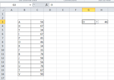
Here this function is showing the result. I hope you like my post. Don’t forget to comment and share it.
Related video tutorials:
Hi! I am Pushpendu. I am the founder and author of Excelabcd. I am little creative person, blogger and Excel-maniac guy. I hope you enjoy my blog.