Lesson#118: Format only cells that contain Conditional Formatting

Have you seen this Conditional Formatting option – Format only cells that contain?

If not then you must remember that this option makes many works of yours easier with Conditional Formatting.

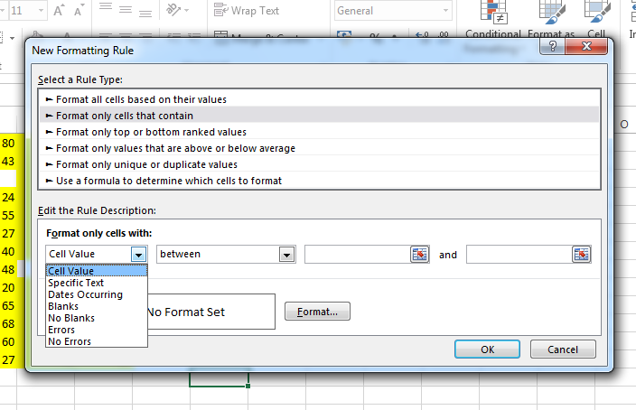
Then you need to go to Conditional Formatting>New Rule

Then select Format only cells that contain

This feature allows you to Highlight

1. Cell values within a specific range
2. Specific Text
3. Dates occurring (example: Yesterday, Today, Tomorrow, Last month, next week, etc.)
4. Blanks
5. No Blanks
6. Errors
7. No Errors

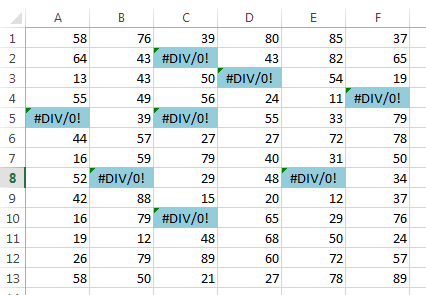
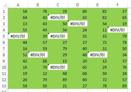
How to highlight errors only

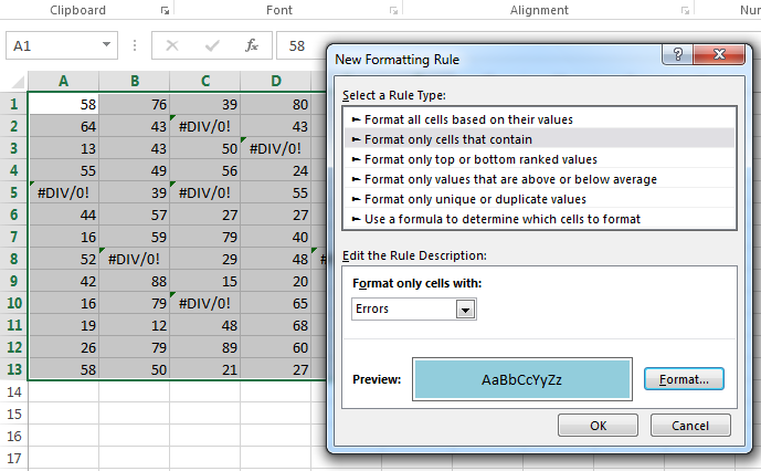
• Select the areas where you want to apply Conditional Formatting
• Then you need to go to Conditional Formatting>New Rule
• Then select Format only cells that contain
• Set a format
• Select the option Errors

How to highlight no errors only

• Select the areas where you want to apply Conditional Formatting
• Then you need to go to Conditional Formatting>New Rule
• Then select Format only cells that contain
• Set a format
• Select the option No errors

How to highlight blanks only

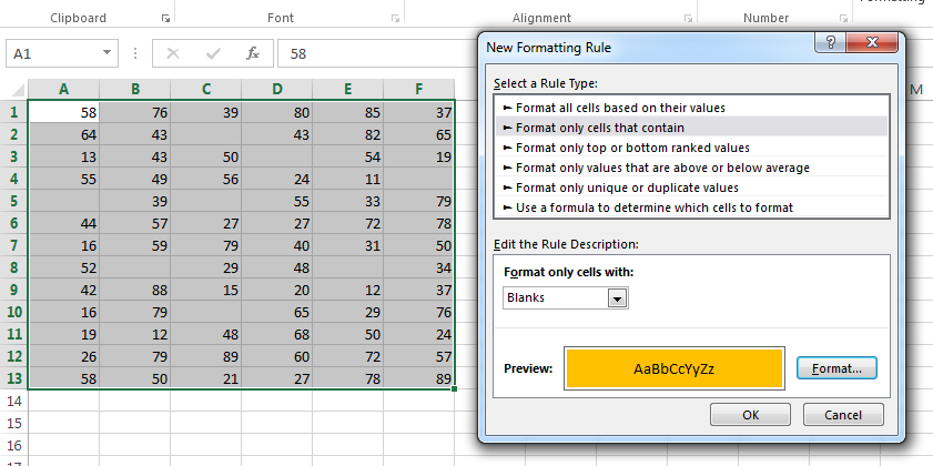
• Select the areas where you want to apply Conditional Formatting
• Then you need to go to Conditional Formatting>New Rule
• Then select Format only cells that contain
• Set a format
• Select the option Blanks

How to highlight no blanks only

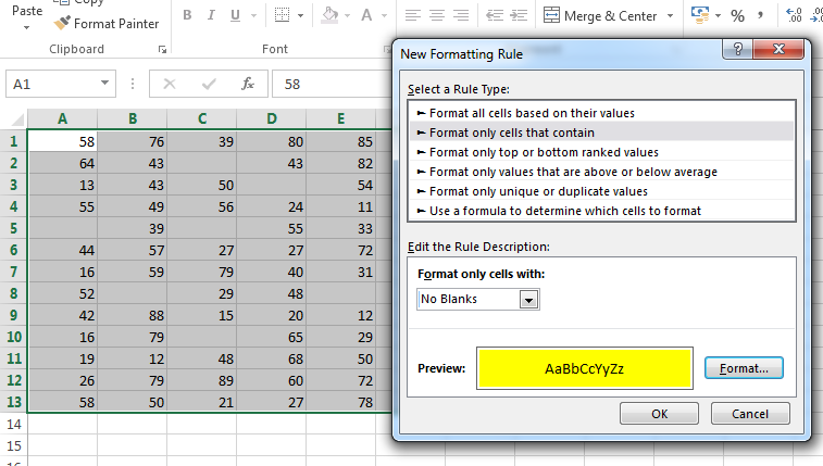
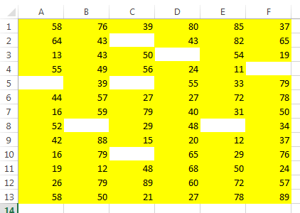
• Select the areas where you want to apply Conditional Formatting
• Then you need to go to Conditional Formatting>New Rule
• Then select Format only cells that contain
• Set a format
• Select the option No blanks