Lesson#140: Color cells if cell value found in another column – Conditional formatting

Here I will make a formula in Conditional Formatting. This formula will color cells if the cell value is found in another column. For example, I am showing this picture below.
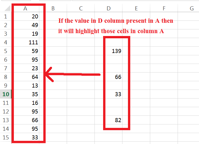
If the value is present in column A then it will color cells in column A.
For that I have to select column A, then I will go to Conditional Formatting>New Rule>Use a formula to determine which cells to format. There I will select a format to highlight and Put the formula.
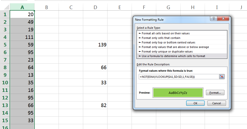
=NOT(ISNA(VLOOKUP($A1,$D:$D,1,FALSE)))
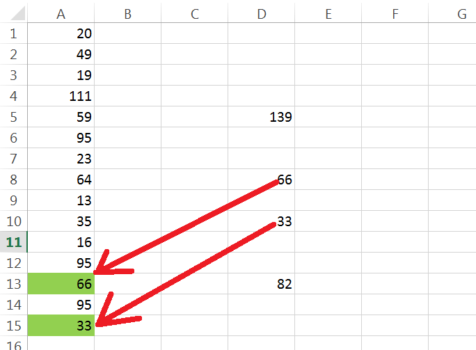
Now this formula will color cells whose values are present in column D.
Hi! I am Pushpendu. I am the founder and author of Excelabcd. I am little creative person, blogger and Excel-maniac guy. I hope you enjoy my blog.
interesting.
I have made one, using formula
(–ISNUMBER(SEARCH,(C1, C4:D20, $C4) and it works
Yes. right.