Lesson#128: Formula to make serial no auto arranged when filtered

Here I will show how to make auto arranged serial no when you filter a column. This post will be very useful to many excel users like me.

Suppose you are using a data sheet and you need to filter certain portions to make a printout. When you filter the data, the serial number becomes the haphazard way. To sort out this problem I have made a simple formula to auto arrange the serial no. Here is a simple example for you.

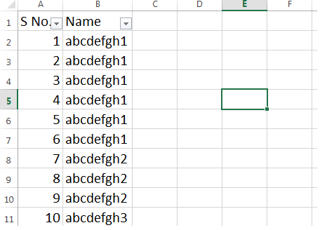
Here in the above picture, I have made two example columns. The first column is serial no and the second one is for content or name. Added a filter on these two columns.

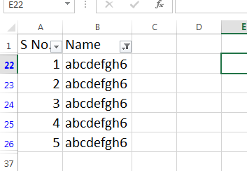
I need to make a formula to auto arrange the serial no like this.

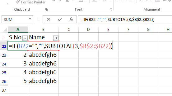
So I have used a simple formula in place of serial no.

=IF(B2=””,””,SUBTOTAL(3,$B$2:$B2))

This formula is placed in the serial no column and it will be dragged down from the first cell to the last cell. Now, whenever you filter the sheet then the serial no will be automatically arranged to start from 1.