Excel TRANSPOSE function

Function              TRANSPOSE

Description        Excel TRANSPOSE function flips the orientation of cells in array mean rows converted to columns and columns converted to rows.

Syntax  TRANSPOSE(array)

array  Mandatory. A reference to a cell or range of cells or an array.

Example:

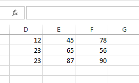
Here I am having an 3×3 array. I am going to transpose this array.

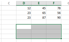
For making it transpose I have to select same 3×3 area in other area of sheet.

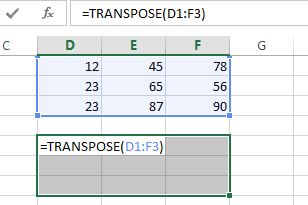
Then I have to write this formula =TRANSPOSE(D1:F3) and then I have to press Ctrl+Shift+Enter

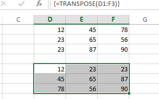
It adds a {=TRANSPOSE(D1:F3)} curly bracket to function This is how array functions works.

Usage Notes:

• When array is transposed, the first row of array becomes the first column of the new array, the second row of array becomes the second column of the new array and so on that’s how it transpose.
• You have to enter the TRANSPOSE function as an array formula that contains same number of cells as array, which means during transpose select same columns for new array as same row numbers in old array and vice versa. Enter the formula by hitting Ctrl + Shift + Enter.
• You can use paste special > transpose for doing the same.

Related Video Tutorials: