Lesson#107: How did I add MS Project features to the Excel project schedule
Here I will discuss a long topic about Excel Gantt chart making. I will show how I made my excel chart work like the ms project schedule by adding some basic features.
Some basic features of the ms project which I added are.
- Auto updating chart month-wise.
- Easy calculation of working days by considering holidays, and weekends.
- Showing related activities. Start to Start, Finish to Start separately.
1. Auto updating chart month-wise.
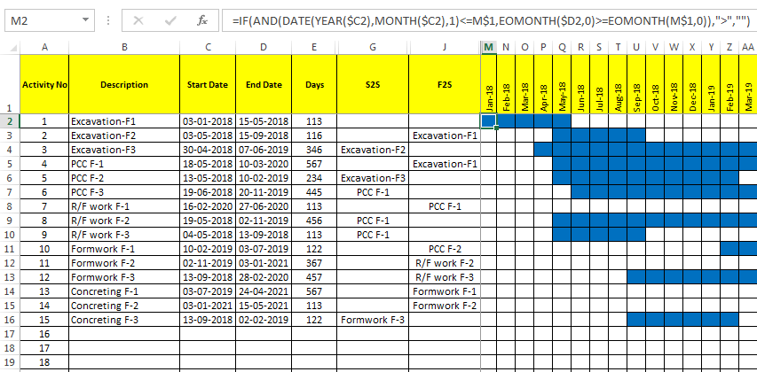
For making a month-wise scheduling chart I made the date format above the Gantt chart area by “mmm-yy” from FormatCells>Custom and drag them up to the requirement.
I will add this formula to show the automatic updating Gantt chart bar
=IF(AND(DATE(YEAR($D2),MONTH($D2),1)<=G$1,EOMONTH($E2,0)>=EOMONTH(G$1,0)),”>”,””)
and I will drag it up to the last.
Now I will select the area of the Gantt chart and put this Formatting from ConditionalFormatting>Highlight Cells Rules>Text that Contains.
I will format the area for “>” this character and I will choose the Fill color and text color the same.
Click to read the related posts.
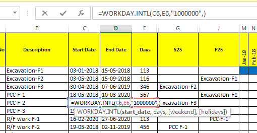
2. Easy calculation of working days by considering holidays, and weekends.
For making a project schedule that considers weekends, and holidays and calculates working day easily I have used
WORKDAY.INTL function.
3. Showing related activities. Start to Start, Finish to Start separately.
For showing the related activities, Start to Start and Finish to Start separately I had to make some extra columns.
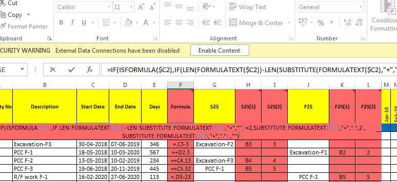
I extracted the formula as text and modified it where I have put the relationship with other activities.
=IF(ISFORMULA($C2),IF(LEN(FORMULATEXT($C2))-LEN(SUBSTITUTE(FORMULATEXT($C2),”+”,””))=2,SUBSTITUTE(FORMULATEXT($C2),”+”,”.”,2),SUBSTITUTE(FORMULATEXT($C2),”+”,”.”)),””)
This formula converts the formula of relation in text and modifies it by converting the second “+” into “.”
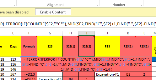
Now I have to extract the row number where I related it and I will distribute it in two columns, S2S and F2S.
For this, I have put the formula in the S2S column.
=IFERROR(IFERROR(IF(COUNTIF($F2,”*C*”),MID($F2,FIND(“C”,$F2)+1,FIND(“.”,$F2)-FIND(“C”,$F2)-1),””),MID($F2,FIND(“C”,$F2)+1,FIND(“-“,$F2)-FIND(“C”,$F2)-1)),MID($F2,FIND(“C”,$F2)+1,4))
And in the F2S column, I have put this formula.
=IFERROR(IFERROR(IF(COUNTIF($F2,”*D*”),MID($F2,FIND(“D”,$F2)+1,FIND(“.”,$F2)-FIND(“D”,$F2)-1),””),MID($F2,FIND(“D”,$F2)+1,FIND(“-“,$F2)-FIND(“D”,$F2)-1)),MID($F2,FIND(“D”,$F2)+1,4))
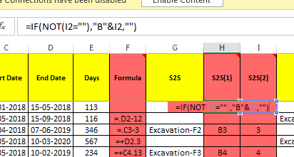
Now the next steps are very easy I have to return the B column values which have the name of the activity. So for S2S column =IF(NOT(I2=””),”B”&I2,””) and for F2S column =IF(NOT(L2=””),”B”&L2,””)
This formula creates the address as text values of the related activity.
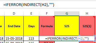
There is a very good function in Excel that takes the input of reference to a cell and returns the value of reference. And this function is INDIRECT.
So by adding these basic features I have made my program schedule in excel more like ms Project.
Download the sheet
NB:- These formulas are compatible with Excel 2013 and higher versions.
Hi! I am Puspendu. I am the founder and author of Excelabcd. I am little creative person, blogger and Excel-maniac guy. I hope you enjoy my blog.